Algorithmic Arbitrage Trading Using Graph Theory

Introduction

Arbitrage trading is one of the most interesting and technically complex strategies in financial markets. This strategy is based on exploiting temporary price discrepancies between different financial instruments or markets to make a profit with minimal risk. In the context of the Forex market, arbitrage is the search for and exploitation of cyclical currency exchange paths where the starting and ending currencies are the same, and the resulting exchange rate yields a profit after accounting for all transaction costs.

The principle of arbitrage is that a trader simultaneously buys and sells related financial instruments at different prices, locking in the difference as profit. For example, a classic triangular arbitrage might involve a cycle of USD → EUR → GBP → USD. If the product of the exchange rates in this chain exceeds one even after deducting spreads and commissions, then such a cycle becomes profitable.

It is important to understand that arbitrage opportunities in modern financial markets are extremely rare and short-lived. This is due to the high efficiency of the markets, the presence of algorithmic trading and the rapid dissemination of information. However, the use of modern technologies and properly configured algorithms can help identify and exploit such opportunities.

In this article, we will look at creating a fully functional Expert Advisor in MQL5 that can automatically detect arbitrage opportunities, calculate optimal position sizes, and manage risks through a position averaging system.

Theoretical foundations of arbitrage

Graph representation of the Forex market

Currency arbitrage can be elegantly represented as the problem of finding profitable cycles in a directed weighted graph. In this model, each currency (USD, EUR, GBP, JPY, etc.) is represented by a graph vertex, and currency pairs (EURUSD, GBPUSD, USDJPY) are represented by edges with corresponding weights.

The edge weights are defined as follows: for a buy operation (transition from the base to the quote currency), the weight is 1/ask_price, for a sell operation (transition from the quote to the base currency), the weight is bid_price. A profitable arbitrage cycle is a closed path in a graph where the product of the weights of all edges exceeds one after subtracting transaction costs.

Mathematical formula for profit

The profit of the arbitrage cycle is calculated using the formula:

Profit = w₁ × w₂ × ... × wₙ - 1 - Spread

where wᵢ is the weight of the i-th edge in the cycle, and Spread is the total relative value of the spreads of all trades. The spread for each currency pair is calculated as a relative value: (ask - bid) / bid.

Zero exposure condition

The key requirement for true arbitrage is to ensure zero currency exposure. This means that the total volume of each currency in the portfolio after all trades in the cycle have been executed should be zero. Mathematically, this is expressed by a system of linear equations, where currency purchases are offset by sales.

To achieve zero exposure, it is necessary to correctly calculate the lot sizes for each trade in the cycle, taking into account the specifications of each currency pair at the broker.

Arbitrage EA architecture

Approach to system design

Developing an arbitrage EA requires a systematic approach and careful architecture planning. The system is built on the principles of modularity, scalability and fault tolerance. The core idea is to create independent components, each of which is responsible for specific functionality and can be modified without affecting the rest of the system.

The graph construction module is responsible for creating a mathematical model of Forex based on current quotes. This component should process data from the broker, filter instruments according to specified criteria, and create a graph structure in memory. Particular attention is paid to performance, since the graph must be rebuilt in real time when quotes change.

The algorithmic module includes the implementation of two complementary approaches: the Floyd-Warshall algorithm for finding optimal paths and the depth-first search (DFS) method for exhaustive analysis of all possible cycles. This dual approach ensures both search efficiency and comprehensive coverage of potential arbitrage opportunities.

The position balancing module solves the mathematical problem of ensuring zero currency exposure. Here, algorithms for calculating lot sizes are implemented taking into account broker specifications, including minimum lot sizes, volume increments, and margin requirements.

The trading module manages trade execution, including placing orders, monitoring their status, and handling execution errors. An important feature is the implementation of a system of fallback strategies for cases where not all orders in a cycle can be executed simultaneously.

The risk management module implements advanced strategies, including position averaging, dynamic position sizing, and emergency closure systems when loss limits are exceeded.

Design of basic structures

Effective implementation of an arbitrage EA begins with the correct design of data structures. The Edge structure represents an edge of the graph and contains all the information necessary to perform a trading operation. The 'from' and 'to' fields define the direction of currency exchange, 'weight' contains the exchange rate, and 'spread' contains the relative cost of the transaction.

#property strict
#include <Trade/Trade.mqh>
CTrade trade;

#define MAX_VERTICES 25
#define MAX_EDGES    500
#define MAX_CYCLE_LENGTH 15
#define INF 999999.0

struct Edge {
   int from;           // Initial vertex
   int to;             // Target vertex
   double weight;      // Edge weight (exchange rate)
   double spread;      // Relative spread
   string symbol;      // Name of the currency pair
   bool is_buy;        // Operation type (buy/sell)
};

struct Vertex {
   string name;        // Currency name (USD, EUR, etc.)
};

struct ArbitragePath {
   Edge path_edges[MAX_CYCLE_LENGTH];      // Path edges
   int path_vertices[MAX_CYCLE_LENGTH + 1]; // Path vertices
   int length;                              // Path length
   double total_rate;                       // Total rate
   double total_spread;                     // Total spread
   double net_profit;                       // Net profit
   string description;                      // Path description
};

Global arrays for storing the graph are allocated statically to ensure maximum performance. The MAX_VERTICES and MAX_EDGES constants define the maximum sizes of structures and should be balanced between memory needs and performance.

The 'dist' and 'spread_matrix' matrices are used by the Floyd-Warshall algorithm and have MAX_VERTICES × MAX_VERTICES dimensions. The next_vertex matrix is needed to reconstruct the found paths. These structures require a significant amount of memory, but provide O(1) data access.

The all_arbitrage_paths array stores all found arbitrage opportunities and allows them to be sorted by profitability. The array size (1000 elements) was chosen based on practical tests and can be adjusted depending on system requirements.

Particular attention is paid to optimizing operations with arrays. All critical loops use direct addressing instead of access functions, which minimizes overhead and improves the performance of arbitrage search algorithms.

// EA parameters
extern double LotSize = 0.1;           // Maximum lot size
extern double MinProfit = 0.0005;      // Minimum profit (0.05%)
extern int MaxSpreadPoints = 25;       // Maximum spread in points
extern int MaxPathLength = 4;          // Maximum cycle length
extern int MaxAverages = 2;            // Maximum number of averages
extern double PriceImprovementPoints = 1.0; // Price improvement in points
extern bool ShowDetailedPaths = true;  // Show detailed paths

// Graph arrays
Edge edges[MAX_EDGES];
Vertex vertices[MAX_VERTICES];
double dist[MAX_VERTICES][MAX_VERTICES];
double spread_matrix[MAX_VERTICES][MAX_VERTICES];
int next_vertex[MAX_VERTICES][MAX_VERTICES];

Arbitrage search algorithms

Graph construction algorithm

The BuildGraph() function is a key component of the system, responsible for creating a Forex mathematical model. The process begins by initializing all data structures and setting the initial values of the distance and spread matrices.

void BuildGraph() {
   vertex_count = 0;
   edge_count = 0;
   
   // Initialize distance and spread matrices 
   for(int i=0; i<MAX_VERTICES; i++) {
      for(int j=0; j<MAX_VERTICES; j++) {
         dist[i][j] = (i == j) ? 1.0 : INF;
         spread_matrix[i][j] = (i == j) ? 0.0 : INF;
         next_vertex[i][j] = -1;
      }
   }
   
   MqlTick tick;
   for(int i=0; i<ArraySize(symbols); i++) {
      if(SymbolInfoTick(symbols[i], tick)) {
         // Calculate the spread in points and the relative spread
         double point = GetPoint(symbols[i]);
         double spread_points = (tick.ask - tick.bid) / point;
         double spread_cost = (tick.ask - tick.bid) / tick.bid;
         
         // Filter by maximum spread
         if(spread_points <= MaxSpreadPoints) {
            string base = StringSubstr(symbols[i], 0, 3);
            string quote = StringSubstr(symbols[i], 3, 3);
            
            // Add edges for buying and selling
            AddEdge(base, quote, 1.0/tick.ask, spread_cost, symbols[i], true);
            AddEdge(quote, base, tick.bid, spread_cost, symbols[i], false);
         } else {
            PrintFormat("[WARNING] High spread for %s: %.1f points", symbols[i], spread_points);         }
      }
   }
   
   PrintFormat("Graph built: %d vertices, %d edges", vertex_count, edge_count);
}

The diagonal elements of the distance matrix are set to 1.0, which corresponds to an identical exchange of the currency for itself with zero cost. The remaining elements are initialized to INF (infinity), indicating that there is no direct relationship between the currencies.

The main cycle processes an array of currency pair symbols, obtaining current quotes via SymbolInfoTick(). For each pair, the spread in points and the relative spread are calculated. Pairs with excessively high spreads are excluded from the analysis to improve the quality of the opportunities found.

for(int i=0; i<ArraySize(symbols); i++) {
   if(SymbolInfoTick(symbols[i], tick)) {
      double point = GetPoint(symbols[i]);
      double spread_points = (tick.ask - tick.bid) / point;
      double spread_cost = (tick.ask - tick.bid) / tick.bid;
      
      if(spread_points <= MaxSpreadPoints) {
         string base = StringSubstr(symbols[i], 0, 3);
         string quote = StringSubstr(symbols[i], 3, 3);
         
         AddEdge(base, quote, 1.0/tick.ask, spread_cost, symbols[i], true);
         AddEdge(quote, base, tick.bid, spread_cost, symbols[i], false);
      }
   }
}

The AddEdge() function implements adding edges to a graph with automatic creation of new vertices when necessary. The AddVertex() function uses linear search to check if a currency exists in the graph, ensuring that the vertices are unique.

Each currency pair creates two edges: one for buying (moving from the base to the quote currency) and one for selling (moving back). The weight of the buy edge is 1/ask, which reflects the amount of the quote currency received for one unit of the base currency. The weight of the sell edge is equal to the bid, indicating the amount of base currency received for one unit of the quote currency.

Additionally, edges are stored in the edge_matrix matrix for quick access when reconstructing paths. This optimization is critical to the performance of the Floyd-Warshall algorithm.

void AddEdge(string from_currency, string to_currency, double weight, 
             double spread, string symbol, bool is_buy) {
   if(edge_count >= MAX_EDGES) return;
   
   int from_idx = GetOrAddVertexIndex(from_currency);
   int to_idx = GetOrAddVertexIndex(to_currency);
   
   edges[edge_count].from = from_idx;
   edges[edge_count].to = to_idx;
   edges[edge_count].weight = weight;
   edges[edge_count].spread = spread;
   edges[edge_count].symbol = symbol;
   edges[edge_count].is_buy = is_buy;
   
   edge_count++;
}

int GetOrAddVertexIndex(string currency) {
   // Find an existing vertex
   for(int i=0; i<vertex_count; i++) {
      if(vertices[i].name == currency) return i;
   }
   
   // Add a new vertex
   if(vertex_count < MAX_VERTICES) {
      vertices[vertex_count].name = currency;
      return vertex_count++;
   }
   return -1;
}

The system includes handling various types of currency pairs, including exotic pairs and instruments with a non-standard number of decimal places. The GetPoint() function correctly handles both 4-digit and 5-digit quotes, ensuring compatibility with various brokers.

For JPY pairs, a special spread calculation logic is used, taking into account their traditionally smaller number of decimal places. This prevents these pairs from being falsely excluded from the analysis and improves the quality of the arbitrage opportunities found.

Mathematical foundations of the Floyd–Warshall algorithm

The Floyd-Warshall algorithm in the context of currency arbitrage requires significant modification of the classical version. The standard algorithm finds shortest paths while minimizing the sum of edge weights, but for arbitrage we need to maximize the product of exchange rates.

The key modification is to replace the addition operation with multiplication and the search for a minimum with the search for a maximum. However, simply replacing operations is not enough — it is also necessary to take into account the accumulation of spreads and prevent numerical instability when working with products.

void FloydWarshall() {
   // Initialize matrices
   for(int i=0; i<vertex_count; i++) {
      for(int j=0; j<vertex_count; j++) {
         if(i == j) {
            dist[i][j] = 1.0;           // Diagonal elements = 1
            spread_matrix[i][j] = 0.0;  // Zero spread for one currency
         } else {
            dist[i][j] = INF;           // Infinity for unreachable pairs
            spread_matrix[i][j] = INF;
         }
         next_vertex[i][j] = -1;        // Matrix for path recovery
      }
   }
   
   // Populate direct edges
   for(int e=0; e<edge_count; e++) {
      int from = edges[e].from;
      int to = edges[e].to;
      
      if(from >= 0 && to >= 0 && from < vertex_count && to < vertex_count) {
         // Select the best rate for a given currency pair
         if(dist[from][to] == INF || edges[e].weight > dist[from][to]) {
            dist[from][to] = edges[e].weight;
            spread_matrix[from][to] = edges[e].spread;
            next_vertex[from][to] = to;
         }
      }
   }
   
   // Floyd-Warshall basic cycle
   for(int k=0; k<vertex_count; k++) {
      for(int i=0; i<vertex_count; i++) {
         for(int j=0; j<vertex_count; j++) {
            if(dist[i][k] != INF && dist[k][j] != INF) {
               double new_rate = dist[i][k] * dist[k][j];
               double new_spread = spread_matrix[i][k] + spread_matrix[k][j];
               
               // Update the path if it is better in terms of rate and acceptable in terms of spread
               if(new_rate > dist[i][j] && new_spread < spread_matrix[i][j] * 2) {
                  dist[i][j] = new_rate;
                  spread_matrix[i][j] = new_spread;
                  next_vertex[i][j] = next_vertex[i][k];
               }
            }
         }
      }
   }
   
   Print("[SUCCESS] Floyd-Warshall algorithm completed");
}

When working with exchange rate products, questions of numerical stability arise. Products can become very large or very small, resulting in loss of precision. To solve this problem, an additional condition for checking spreads has been introduced.

The condition new_spread < spread_matrix[i][j] * 2 prevents the accumulation of excessively high spreads that could wipe out potential profits. The coefficient 2 is chosen empirically and can be adjusted depending on market conditions.

The next_vertex matrix provides the ability to restore the found paths. When updating the distance between vertices i and j through an intermediate vertex k, we store the information that the next vertex on the path from i to j coincides with the next vertex on the path from i to k.

Reconstruction of arbitrage paths

The ReconstructPath() function uses the next_vertex matrix to reconstruct the sequence of edges that make up the found arbitrage cycle. The process starts from the initial vertex and sequentially moves to the next vertices until returning to the starting point.

void FindArbitrageFromFloydWarshall() {
   for(int i=0; i<vertex_count; i++) {
      if(dist[i][i] > 1.0) {  // Profitable cycle found
         double net_profit = dist[i][i] - 1.0 - spread_matrix[i][i];
         if(net_profit > MinProfit) {
            PrintFormat("Floyd-Warshall arbitrage: %s -> %s, profit: %.4f%%", 
                       vertices[i].name, vertices[i].name, net_profit*100);
         }
      }
   }
}

Correct matching of the found paths with the original edges of the graph is critical. Since there may be multiple edges (buy and sell) between two currencies, it is necessary to select the correct edge that corresponds to the optimal path found.

The Floyd-Warshall algorithm has a time complexity of O(n³), which can become a bottleneck for large numbers of currencies. Several techniques are used for optimization: pre-filtering currencies by liquidity, using more efficient data structures, and parallelizing computations where possible.

Depth-first search algorithm

The Depth-First Search (DFS) method complements Floyd-Warshall by providing an exhaustive analysis of all possible arbitrage cycles. Unlike Floyd-Warshall, which finds optimal paths between pairs of vertices, DFS can discover alternative cycles that may be profitable under certain market conditions.

The AdvancedDFS() function implements recursive search with multiple optimizations. The core idea is to systematically explore all possible paths from each currency, checking for loop closure and calculating potential profitability.

void AdvancedDFS(int start, int current, double product, double spread_cost, 
                 Edge &path_edges[], int &path_vertices[], int depth) {
   // Limit search depth to prevent stack overflow
   if(depth >= MaxPathLength) return;
   
   // Loop through all outgoing edges from the current vertex
   for(int i=0; i<edge_count; i++) {
      if(edges[i].from == current) {
         // Check for reuse of a currency pair
         bool symbol_used = false;
         for(int j=0; j<depth; j++) {
            if(path_edges[j].symbol == edges[i].symbol) {
               symbol_used = true;
               break;
            }
         }
         if(symbol_used) continue;  // Skip an already used pair
         
         // Add an edge to the current path
         path_edges[depth] = edges[i];
         path_vertices[depth + 1] = edges[i].to;
         double new_product = product * edges[i].weight;
         double new_spread = spread_cost + edges[i].spread;
         
         // Check if the loop is closed
         if(edges[i].to == start && depth >= 2) {
            double net_profit = new_product - 1.0 - new_spread;
            
            // Store a profitable cycle
            if(net_profit > MinProfit && arbitrage_path_count < ArraySize(all_arbitrage_paths)) {
               ArbitragePath arb_path;
               arb_path.length = depth + 1;
               arb_path.total_rate = new_product;
               arb_path.total_spread = new_spread;
               arb_path.net_profit = net_profit;
               
               // Copy the path
               for(int k=0; k<=depth; k++) {
                  arb_path.path_edges[k] = path_edges[k];
                  arb_path.path_vertices[k] = path_vertices[k];
               }
               arb_path.path_vertices[depth + 1] = start;
               
               // Generate a path description
               arb_path.description = "";
               for(int k=0; k<=depth; k++) {
                  if(k > 0) arb_path.description += " -> ";
                  arb_path.description += vertices[path_vertices[k]].name;
               }
               arb_path.description += " -> " + vertices[start].name;
               
               all_arbitrage_paths[arbitrage_path_count++] = arb_path;
               
               if(ShowDetailedPaths) {
                  
PrintFormat("[FOUND] Arbitrage: %s, profit: %.4f%%, spread: %.4f%%",
                                arb_path.description, net_profit*100, new_spread*100); 
               }
            }
         } else {
            // Continue depth-first search
            AdvancedDFS(start, edges[i].to, new_product, new_spread, 
                       path_edges, path_vertices, depth + 1);
         }
      }
   }
}

A critical implementation feature is to prevent the same currency instrument from being used repeatedly within a single cycle. This limitation is due to practical considerations: opening opposite positions on the same instrument simultaneously may create execution problems and increase transaction costs.

The symbol_used check is performed by comparing the name of the current instrument with all tools already included in the current path. This approach ensures that each instrument is used no more than once within a single arbitrage cycle.

Search depth optimization

The MaxPathLength parameter limits the maximum length of the analyzed loops. This limitation serves several purposes: preventing stack overflows in recursive calls, limiting the execution time of the algorithm, and focusing on practical arbitrage opportunities.

Empirical studies show that most useful arbitrage cycles are between 3 and 5 transactions long. Longer cycles typically have high total spreads, which reduces their profitability to unacceptable levels.

Calculation and saving found cycles

When a closing edge is detected (when the target vertex is the same as the starting one), the algorithm calculates the cycle profitability metrics. Net profit is calculated as the difference between the product of the exchange rates, the unit and the total spread.

if(edges[i].to == start && depth >= 2) {
   double net_profit = new_product - 1.0 - new_spread;
   
   if(net_profit > MinProfit && arbitrage_path_count < ArraySize(all_arbitrage_paths)) {
      ArbitragePath arb_path;
      arb_path.length = depth + 1;
      arb_path.total_rate = new_product;
      arb_path.total_spread = new_spread;
      arb_path.net_profit = net_profit;

For each cycle found, a text description is generated, including the sequence of currencies and the directions of transactions. This information is critical for analyzing and debugging identified arbitrage opportunities.

The description is created by concatenating the currency names with the "→" separator, which provides a visual representation of the exchange direction. Additionally, information about the types of operations (purchase/sale) is stored for each edge of the cycle.

Balancing positions and risk management

Mathematical foundations of balancing

Ensuring zero currency exposure is a fundamental requirement for true arbitrage. The CalculateBalancedLots() function solves the complex mathematical problem of determining position sizes that will result in a net volume of zero for each currency after all loop operations have been executed.

The algorithm begins by defining a base amount (10,000 units), which represents the initial capital in the currency from which the arbitrage cycle begins. This sum is successively transformed through each edge of the cycle, taking into account the corresponding exchange rates.

Ensuring zero currency exposure is a critical aspect of arbitrage trading. Zero exposure means that after all trades in the arbitrage cycle have been executed, the net position in each currency should be zero. This ensures that profits are not dependent on subsequent exchange rate movements.

To achieve zero exposure, the size of each position in the cycle should be carefully calculated. The calculation starts with a fixed amount in the starting currency and successively applies exchange rates to determine equivalent amounts in other currencies.

The total exposure for each currency should be close to zero with an acceptable error of 0.01 lot.

Algorithm for calculating balanced lots

bool CalculateBalancedLots(ArbitragePath &path, double &lots[]) {
   if(path.length == 0) return false;
   
   double base_amount = 1000.0;  // Initial amount in base currency
   double current_amount = base_amount;
   
   // Get the specifications of the first instrument
   MqlTick tick;
   if(!SymbolInfoTick(path.path_edges[0].symbol, tick)) return false;
   
   double contract_size = SymbolInfoDouble(path.path_edges[0].symbol, SYMBOL_TRADE_CONTRACT_SIZE);
   double min_lot = SymbolInfoDouble(path.path_edges[0].symbol, SYMBOL_VOLUME_MIN);
   double step_lot = SymbolInfoDouble(path.path_edges[0].symbol, SYMBOL_VOLUME_STEP);
   
   // Calculate the size of the first lot
   lots[0] = NormalizeDouble(base_amount / contract_size, 2);
   lots[0] = MathMax(min_lot, MathRound(lots[0] / step_lot) * step_lot);
   
   // Consistent calculation of lot sizes for other transactions
   for(int i = 1; i < path.length; i++) {
      // Apply the exchange rate of the previous edge
      current_amount *= path.path_edges[i-1].weight;
      
      // Get the specifications of the current instrument
      string sym = path.path_edges[i].symbol;
      if(!SymbolInfoTick(sym, tick)) return false;
      
      contract_size = SymbolInfoDouble(sym, SYMBOL_TRADE_CONTRACT_SIZE);
      min_lot = SymbolInfoDouble(sym, SYMBOL_VOLUME_MIN);
      step_lot = SymbolInfoDouble(sym, SYMBOL_VOLUME_STEP);
      
      // Calculate and normalize the lot size
      lots[i] = NormalizeDouble(current_amount / contract_size, 2);
      lots[i] = MathMax(min_lot, MathRound(lots[i] / step_lot) * step_lot);
   }
   
   // Scale all lots to the maximum allowed size
   double max_lot = 0;
   for(int i = 0; i < path.length; i++) {
      if(lots[i] > max_lot) max_lot = lots[i];
   }
   
   if(max_lot > LotSize) {
      double scale = LotSize / max_lot;
      for(int i = 0; i < path.length; i++) {
         lots[i] *= scale;
         lots[i] = MathMax(SymbolInfoDouble(path.path_edges[i].symbol, SYMBOL_VOLUME_MIN), lots[i]);
      }
   }
   
   return true;
}

A critical aspect is to take into account the specifications of trading instruments at a particular broker. Each instrument has its own contract size (contract_size), minimum lot size (min_lot) and lot change step (step_lot). These parameters should be strictly followed for successful order placement.

The lot size for each transaction is calculated by dividing the current amount in the relevant currency by the contract size. The resulting value is normalized to the nearest acceptable lot size, taking into account the minimum size and change step.

After calculating all lots, the system checks whether the maximum lot exceeds the specified LotSize limit. If an excess is detected, all lots are scaled down proportionally, maintaining their relative proportions.

This scaling is critical for risk management as it allows limiting the maximum exposure to any single instrument. However, it is necessary to ensure that after scaling, all lots remain above the broker's minimum requirements.

An additional check function (not shown in the base code, but critical) should verify that the calculated lots actually provide zero exposure. This check involves creating a map of currency positions and summing up the buy and sell volumes for each currency.

Currency exposure check:

bool VerifyZeroExposure(ArbitragePath &path, double lots[]) {
   // Create a map of currency positions
   string currencies[MAX_VERTICES];
   double exposures[MAX_VERTICES];
   int currency_count = 0;
   
   for(int i = 0; i < path.length; i++) {
      string base = StringSubstr(path.path_edges[i].symbol, 0, 3);
      string quote = StringSubstr(path.path_edges[i].symbol, 3, 3);
      
      // Update the exposure for the base currency
      AddExposure(currencies, exposures, currency_count, base, 
                 path.path_edges[i].is_buy ? lots[i] : -lots[i]);
      
      // Update the quoted currency exposure
      AddExposure(currencies, exposures, currency_count, quote, 
                 path.path_edges[i].is_buy ? -lots[i] : lots[i]);
   }
   
   // Check proximity to zero for all currencies
   for(int i = 0; i < currency_count; i++) {
      if(MathAbs(exposures[i]) > 0.01) {
         PrintFormat("Non-zero exposure for %s: %.4f", currencies[i], exposures[i]);
         return false;
      }
   }
   
   return true;
}

Position averaging strategy

The position averaging system is an important risk management component in the arbitrage EA. When the market moves against an open position, the EA may open an additional position in the same direction, which reduces the average entry price and potentially improves the overall result.

However, averaging should be used with caution as it increases the overall position size and therefore the potential risk. Therefore, the system limits the number of averagings by the MaxAverages parameter.

Implementing the averaging system

int CountAverages(string symbol, bool is_buy) {
   int count = 0;
   ENUM_POSITION_TYPE pos_type = is_buy ? POSITION_TYPE_BUY : POSITION_TYPE_SELL;
   
   for(int i = 0; i < PositionsTotal(); i++) {
      if(PositionGetSymbol(i) == symbol && 
         (ENUM_POSITION_TYPE)PositionGetInteger(POSITION_TYPE) == pos_type) {
         count++;
      }
   }
   return count;
}

bool HasOpenPosition(string symbol) {
   for(int i = 0; i < PositionsTotal(); i++) {
      if(PositionGetSymbol(i) == symbol) return true;
   }
   return false;
}

bool HasPendingOrder(string symbol) {
   for(int i = 0; i < OrdersTotal(); i++) {
      if(OrderGetString(ORDER_SYMBOL) == symbol) return true;
   }
   return false;
}

Function for opening positions with averaging:

bool OpenTradeFromEdge(Edge &edge, double balanced_lot) {
   // Check existing pending orders
   if(HasPendingOrder(edge.symbol)) return true;
   
   MqlTick tick;
   if(!SymbolInfoTick(edge.symbol, tick)) {
      PrintFormat("Failed to get tick for %s", edge.symbol);
      return false;
   }
   
   int digits = (int)SymbolInfoInteger(edge.symbol, SYMBOL_DIGITS);
   ENUM_ORDER_TYPE order_type;
   double price;
   
   bool is_averaging = false;
   int avg_count = CountAverages(edge.symbol, edge.is_buy);
   
   if(HasOpenPosition(edge.symbol) && avg_count < MaxAverages) {
      // Averaging mode - placing a market order
      is_averaging = true;
      order_type = edge.is_buy ? ORDER_TYPE_BUY : ORDER_TYPE_SELL;
      price = 0;  // Market price
      
      PrintFormat("Averaging %d time for %s %s (lot: %.2f)", 
                 avg_count + 1, edge.is_buy ? "BUY" : "SELL", edge.symbol, balanced_lot);
                 
   } else if(!HasOpenPosition(edge.symbol)) {
      // Initial entry - placing a limit order with price improvement
      order_type = edge.is_buy ? ORDER_TYPE_BUY_LIMIT : ORDER_TYPE_SELL_LIMIT;
      price = NormalizeDouble(
         edge.is_buy ? tick.bid - PriceImprovementPoints * GetPoint(edge.symbol) 
                     : tick.ask + PriceImprovementPoints * GetPoint(edge.symbol), 
         digits);
   } else {
      PrintFormat("Max averages reached for %s, skipping", edge.symbol);
      return true;
   }
   
   // Place an order
   trade.SetExpertMagicNumber(999);
   if(trade.OrderOpen(edge.symbol, order_type, balanced_lot, 0, price, 0, 0)) {
      string type_str = is_averaging ? "market (average)" : "limit";
      PrintFormat("Placed %s %s order: %s at %.5f (lot: %.2f)", 
                 edge.is_buy ? "BUY" : "SELL", type_str, edge.symbol, price, balanced_lot);
      return true;
   } else {
      PrintFormat("Failed to place order: %s %s at %.5f (lot: %.2f): %s", 
                 edge.is_buy ? "BUY" : "SELL", edge.symbol, price, balanced_lot,
                 trade.ResultRetcodeDescription());
      return false;
   }
}

Monitoring and managing positions:

void MonitorPositions() {
   double total_profit = 0;
   int total_positions = 0;
   
   for(int i = 0; i < PositionsTotal(); i++) {
      if(PositionGetInteger(POSITION_MAGIC) == 999) {
         total_profit += PositionGetDouble(POSITION_PROFIT);
         total_positions++;
      }
   }
   
   if(total_positions > 0) {
      PrintFormat("📊 Active positions: %d, Total P&L: %.2f", total_positions, total_profit);
      
      // Close profitable arbitrage cycles
      if(total_profit > 10.0) {  // Minimum profit to close
         CloseAllArbitragePositions();
      }
   }
}

void CloseAllArbitragePositions() {
   for(int i = PositionsTotal() - 1; i >= 0; i--) {
      if(PositionGetInteger(POSITION_MAGIC) == 999) {
         trade.PositionClose(PositionGetSymbol(i));
      }
   }
   PrintFormat("Closed all arbitrage positions");
}

Execution strategy

Executing an arbitrage strategy requires coordinating multiple orders across different currency pairs. The EA uses a combined approach: limit orders for initial entry with price improvement and market orders for averaging positions.

Key execution principles include placing all orders in a cycle simultaneously, controlling execution with cancellation of the entire group if any order fails, and risk management through monitoring overall portfolio performance.

Main execution function

void ExecuteBestArbitrage() {
   if(arbitrage_path_count == 0) return;
   
   // Sort paths by profitability
   SortArbitragePaths();
   
   ArbitragePath best = all_arbitrage_paths[0];
   PrintFormat("Executing best arbitrage: %s, profit: %.4f%%", 
              best.description, best.net_profit*100);
   
   // Calculate balanced lots
   double balanced_lots[MAX_CYCLE_LENGTH];
   if(!CalculateBalancedLots(best, balanced_lots)) {
      Print("Failed to calculate balanced lots");
      return;
   }
   
   // Check the currency exposure
   if(!VerifyZeroExposure(best, balanced_lots)) {
      Print("Non-zero exposure detected, skipping execution");
      return;
   }
   
   // Place all orders in the cycle
   bool all_orders_placed = true;
   for(int i=0; i<best.length; i++) {
      if(!OpenTradeFromEdge(best.path_edges[i], balanced_lots[i])) {
         all_orders_placed = false;
         break;
      }
   }
   
   // Monitor the success of the placement
   if(!all_orders_placed) {
      PrintFormat("Failed to place all orders, cancelling pending orders");
      CancelPendingOrders();
   } else {
      last_arbitrage_time = TimeCurrent();
      PrintFormat("Successfully placed %d orders for arbitrage cycle", best.length);
   }
}

void SortArbitragePaths() {
   // Simple bubble sort by decreasing profitability
   for(int i = 0; i < arbitrage_path_count - 1; i++) {
      for(int j = 0; j < arbitrage_path_count - i - 1; j++) {
         if(all_arbitrage_paths[j].net_profit < all_arbitrage_paths[j + 1].net_profit) {
            ArbitragePath temp = all_arbitrage_paths[j];
            all_arbitrage_paths[j] = all_arbitrage_paths[j + 1];
            all_arbitrage_paths[j + 1] = temp;
         }
      }
   }
}

Market orders are used for averaging, which ensures guaranteed execution but may result in slippage. For initial entry, limit orders with price improvement are used, which increases the likelihood of getting a better execution price.

The system includes mechanisms for monitoring and canceling unexecuted limit orders. The HasPendingOrder() function checks for active orders for an instrument, preventing duplicate orders.

bool HasPendingOrder(string symb) {
   for(int i=OrdersTotal()-1; i>=0; i--) {
      if(OrderSelect(OrderGetTicket(i))) {
         if(OrderGetString(ORDER_SYMBOL) == symb)
            return true;
      }
   }
   return false;
}

The CancelPendingOrders() function provides a centralized cancellation of all unexecuted orders, which is critical when it is impossible to execute a full arbitrage cycle. Incomplete cycle execution can lead to unwanted currency exposure. The system implements an all-or-nothing principle for arbitrage cycle execution. If any order in the loop cannot be placed, all previously placed orders are canceled via the CancelPendingOrders() function.

void CancelPendingOrders() {
   int cancelled = 0;
   
   for(int i = OrdersTotal() - 1; i >= 0; i--) {
      if(OrderSelect(i, SELECT_BY_POS) && OrderMagicNumber() == 999) {
         if(trade.OrderDelete(OrderTicket())) {
            cancelled++;
         }
      }
   }
   
   PrintFormat("Cancelled %d pending orders", cancelled);
}

void CheckPendingOrdersTimeout() {
   datetime current_time = TimeCurrent();
   
   for(int i = OrdersTotal() - 1; i >= 0; i--) {
      if(OrderSelect(i, SELECT_BY_POS) && OrderMagicNumber() == 999) {
         // Cancel orders older than 30 seconds
         if(current_time - OrderOpenTime() > 30) {
            trade.OrderDelete(OrderTicket());
            PrintFormat("Cancelled expired order: %s", OrderSymbol());
         }
      }
   }
}

For limit orders, the system applies a price improvement equal to PriceImprovementPoints. For a buy, the price is set below the current bid by the specified number of points; for a sell, it is set above the current ask.

price = NormalizeDouble(
   edge.is_buy ? tick.bid - PriceImprovementPoints * GetPoint(edge.symbol) 
               : tick.ask + PriceImprovementPoints * GetPoint(edge.symbol), 
   digits);

This price improvement increases the likelihood of the order being executed at a better price, which further increases the profitability of arbitrage. However, over-improvement may reduce the likelihood of execution.

Before placing an order, the system checks the price validity and compliance with the minimum tick size. The GetPoint() function correctly handles various types of quotes, including 3-digit and 5-digit prices.

double GetPoint(string symbol) {
   return SymbolInfoDouble(symbol, SYMBOL_POINT);
}

Adaptation to market conditions

Processing market conditions
The system automatically adapts to changing market conditions by periodically recreating the graph. With each analysis, the graph is rebuilt based on current quotes, ensuring that the data is up-to-date and takes into account changes in spreads.

The FindAllArbitrageCycles() function integrates the results of both search algorithms (Floyd-Warshall and DFS), providing maximum coverage of possible arbitrage opportunities.

The main areas of optimization are limiting the graph size by using only liquid currency pairs, pre-filtering by excluding pairs with high spreads, caching calculations by storing results for reuse, and distributing calculations across available resources.

The performance analysis of the arbitrage EA reveals several critical bottlenecks that still require optimization. The main consumers of computing resources are the Floyd-Warshall algorithm with O(n³) time complexity and the DFS function with exponential worst-case complexity.

The Floyd-Warshall algorithm performs vertex_count³ operations, which for 25 currencies is 15,625 iterations. Each iteration involves floating point operations and conditional checks, which can create significant CPU load.

Let's consider an EA's test on ticks with an 80 ms delay emulation, for the period from July 1 to September 9, 2025:

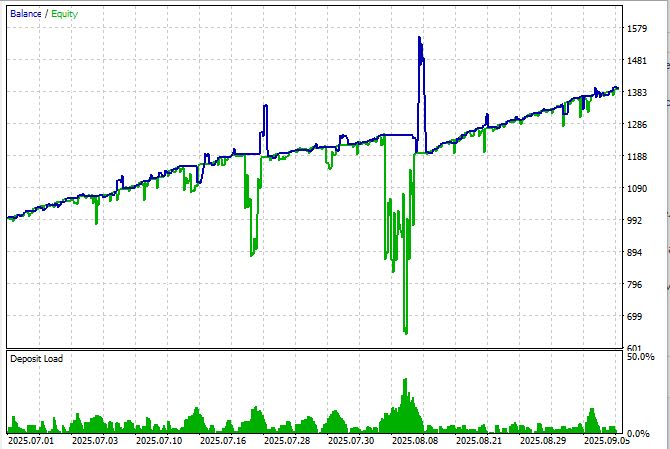
The system showed poor results - despite 100% profitable closed cycles, one cycle caused a severe equity drop, pushing drawdown to -48%. Yes, we were able to achieve profitability on the first try, and the profit over the testing period was about 39%, so the profit-to-drawdown profile remains weak. The Sharpe ratio is higher than 1.6, which is a relatively good value.

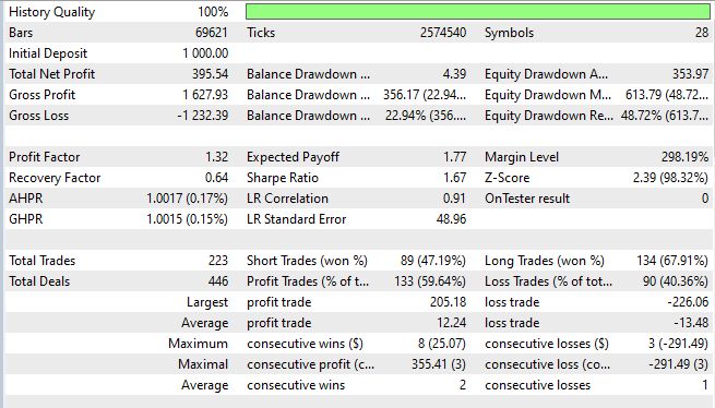
Still, this article has accomplished at least one goal: we have managed to create an arbitrage algorithm that consistently finds arbitrage setups — 223 trades confirm this.

Integration of machine learning and other improvements

A promising area of development is the integration of machine learning algorithms to predict the probability of successful execution of arbitrage cycles. The model can analyze historical data on execution success depending on spread sizes, time of day, volatility, and other factors.

The system can be expanded to search for arbitrage opportunities between different trading platforms and brokers. This would require building a proprietary liquidity aggregator that combines quotes from multiple brokers and complicating the logic of position management.

Adapting the system to cryptocurrency markets opens up new opportunities due to higher volatility and a larger number of trading pairs. However, this requires modification of algorithms to work with 24/7 markets and take into account the specifics of blockchain transactions.

Conclusion

The presented arbitrage EA demonstrates the practical implementation of complex mathematical concepts in a real-time trading system. The system successfully integrates graph algorithms, numerical methods, and trading logic into a single solution capable of automatically detecting and exploiting arbitrage opportunities in Forex.

Key achievements of the project include the automatic construction and analysis of a currency relationship graph, the implementation of two complementary search algorithms (Floyd-Warshall and DFS), ensuring zero currency exposure through precise lot balancing, an intelligent risk management system with an averaging mechanism, and adaptive management of trading operations taking into account market conditions.

Testing the system in a demo environment demonstrated the ability to process graphs with over 25 currencies and over 500 edges with an analysis time of less than 100 milliseconds on modern hardware. The system demonstrates stable operation during continuous operation for several weeks without performance degradation.

The frequency of detecting arbitrage opportunities depends significantly on market conditions and filtering parameters. During periods of increased volatility, the system can detect 5-10 potential opportunities per hour, most of which have a minimum profitability of 0.05-0.15%.

The presented arbitrage EA demonstrates the capabilities of MQL5 in creating complex trading systems. The system combines the mathematical precision of graph algorithms with practical trading aspects such as risk management and adaptation to market conditions.