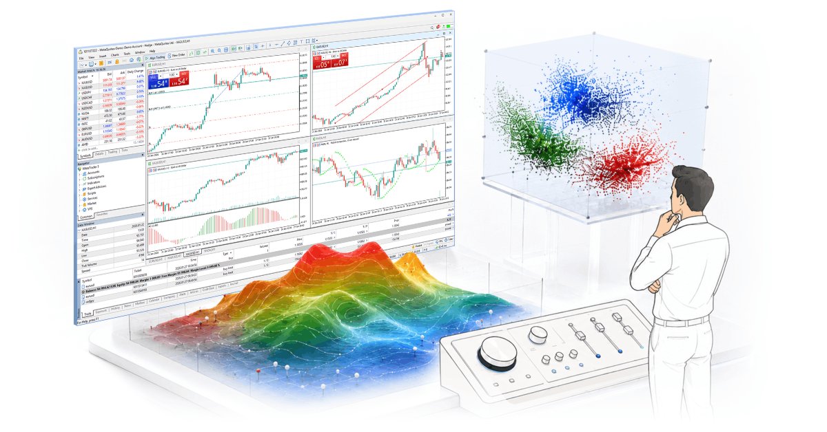
3D Visualization Without External Libraries: How MetaTrader 5 Reveals Optimization Results via MQL5 + DX11

From a beautiful picture to a working tool

When the number of strategy parameters exceeds ten, and the tester's report turns into a multi-page table with numerical series, traders and developers face a problem: the useful signal gets lost in the noise. Flat charts and two-dimensional heat maps are effective up to a certain point, but beyond that, the human brain inevitably trips up due to the multidimensionality of the data. We try to keep in mind the correlation between the indicator period, stop-loss, volatility, and maximum drawdown, but the cognitive load grows faster than the usefulness of the information. 

3D visualization and interactive interfaces in MetaTrader 5 are not an attempt to turn the trading terminal into a gaming engine. This is a technique aimed at reducing cognitive friction. A 3D surface, where the height corresponds to the expected value, and the color gradient reflects drawdown resilience, allows us to highlight the "plateau of stability" and cut off the "needles of overfitting" in seconds. What requires hours of comparison in a tabular format is read as a pattern in three-dimensional space: plane slopes, elevation changes, plateaus/needles, and zones of contrast.

MetaTrader 5 provides a ready-made technological foundation for this task. Native DirectX 11 support, the built-in shader pipeline and the CDXCanvas / CChartObjectDX classes are integrated directly into the MQL5 environment. The developer does not need to connect external graphics libraries, write wrappers in C++, or deal with dependencies: the entire cycle from device creation to frame output is accessible through the standard 3D API, and loading shaders and textures works directly from the Files\DX\ folder.

In this article, we will walk through how to transform optimization result arrays, cluster volumes, and scenario models into manageable 3D landscapes. We will define the criteria of appropriateness: when 3D graphics add signal analysis capabilities, and when they generate visual noise. We will then move on to the architecture of the DX pipeline, examining initialization, binding metrics to vertex buffers, camera mechanics, and UI panels, and finally assessing the technological limitations of the environment.

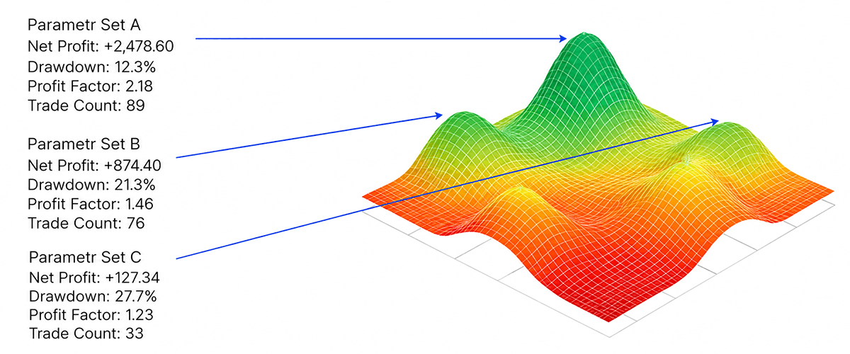
Fig. 1. Text vs. visualization

When 3D and interactivity are really useful

A trader and strategy developer has a powerful, yet often underestimated, tool in their arsenal: visual perception. Report tables, metric lists, and flat graphs do a good job of documenting results. But when it comes to understanding complex relationships, the human brain switches to a different mode: it searches for patterns in the form of images, volume, and context. This is where 3D visualization and interactivity cease to be decoration and become an analytical tool.

Adding a third axis is justified when there is a clear analytical hypothesis in the data. For example, the dependence of the expected value on two key parameters of the system at a fixed risk level. In this case, the 3D surface transforms abstract coordinates into a terrain, where green "mountains" indicate areas of stable profit, and red "dips" indicate drawdowns. The 3D representation acts as a filter: it filters out noise and leaves only those combinations that are meaningful.

Not for aesthetics, but for analytical value

We are not talking about decorative graphics, but about visual layers that directly reveal what is hidden within the optimization report lines. A flat table answers the question: "What is the result of this combination of parameters?"

A 3D surface answers the question: "How does the result change with smooth changes in two parameters, and where are the stability zones?" This is a fundamentally different level of strategy analysis. The stability of the result when the external context changes is the main thing to achieve when testing any idea. Everything else is secondary.

There are at least three scenarios where 3D visualization provides an advantage:

1. Optimization landscape

Imagine that you are selecting two parameters: the moving average period and the stop loss size. In the table, you see 100 rows with Profit and Drawdown values. On a 3D surface with a color gradient, you will instantly see:

• Robustness plateaus are vast green zones where the strategy is consistently profitable even with varying parameters;
• Sharp peaks are narrow local maxima that are often a sign of overfitting;
• Steep slopes are areas where a small change in a parameter results in a sharp increase in drawdown.

This 3D surface allows for informed decisions about choosing a working set of parameters based not on maximum profit, but on robustness.

2. Market condition as a multidimensional space

Clustering market regimes (trend, flat, increased volatility) often requires analyzing more than three indicators simultaneously. Here 3D visualization allows:

• Represent each market state as a point in feature space;
• Color code the effectiveness of the strategy in this mode (this point);
• Interactively rotate the point cloud to reveal hidden groupings.

This is especially convenient when adaptively setting parameters: you can see under what conditions the strategy fails and where it performs robustly.

3. Scenario modeling and stress testing

When running the strategy on a variety of synthetic scenarios (Monte Carlo method, price path generation, questions like: what if volatility increases by 30%?), the 3rd dimension can display:

• X-axis — strategy parameter;
• Y-axis – market stress level (volatility, gaps);
• Z-axis / color — final metric (recovery factor, expected value).

As a result, we are observing not just some worst-case scenario, but the boundary of the strategy’s robustness under deteriorating market conditions.

Selection criteria: When 3D is overkill

Let's formulate a rule: 3D is justified when you are investigating the dependence of a result on two or more continuous variables and it is important for you to see the geometry of this dependence.

If you are ready to try replacing hours of report sifting with intuitive visual analysis, let's start with the rendering pipeline.

Basic DX pipeline in MQL5: From initialization to the first frame

Creating 3D graphics in MetaTrader 5 is a sequential process, where each stage has its own purpose. Understanding the architecture of DirectX objects and the rendering loop allows us to avoid common pitfalls, such as memory leaks, flickering graphics, and performance degradation when working with large amounts of data.

DirectX object architecture in MQL5

The basis of 3D graphics in MQL5 is the CCanvas3D class, which encapsulates all the complexity of working with DirectX 11. It provides a high-level API to the developer, hiding the low-level details of creating devices, contexts, and buffers.

Object hierarchy:

• CCanvas3D — a class that manages the scene, camera, and rendering
• CDXMesh and its descendants (CDXBox, CDXSphere, CDXTorus) — geometric objects
• DXVertex — vertex structure containing coordinates, normals, texture coordinates, and color

struct DXVertex
  {
   DXVector4  position;   // vertex coordinates
   DXVector4  normal;     // normal vector
   DXVector2  tcoord;     // texture coordinates
   DXColor    vcolor;     // color
  };

This structure is compatible with the standard vertex shader, eliminating the need to write custom shaders for basic tasks. For complex projects, we recommend using the methods and utilities presented in the file MQL5\Include\Canvas\DX\DXUtils.mqh.

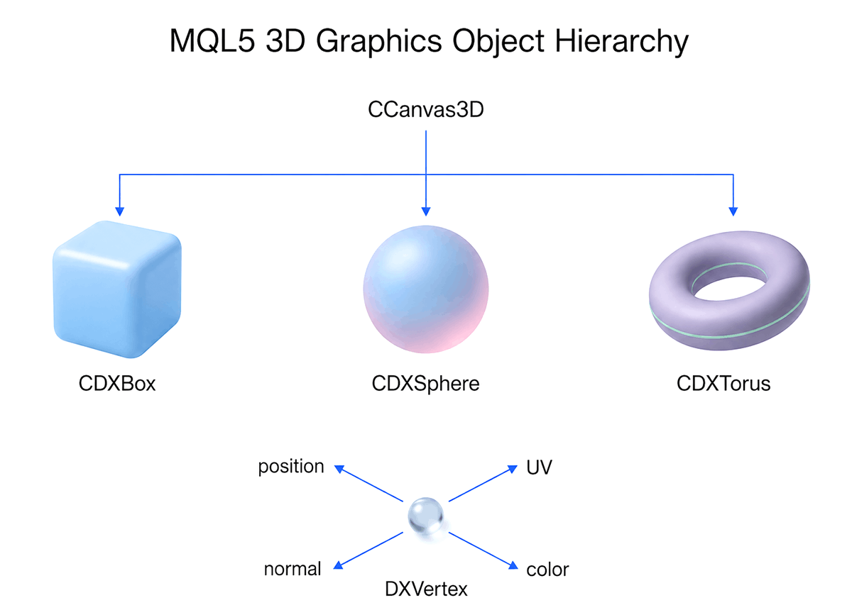
Fig. 2. Hierarchy of 3D graphics in MQL5

All resources (shaders, textures, buffers) are managed via DXDispatcher. Every created object should be explicitly destroyed via Destroy() or Shutdown() in the destructor. MetaTrader 5 does not have a garbage collector for DirectX resources, and memory leaks accumulate until the terminal is restarted.

Pipeline initialization

The first step is to create a canvas and set up the projection matrix:

//+------------------------------------------------------------------+
//+ canvas creation and projection matrix setup                      |
//+------------------------------------------------------------------+
virtual bool Create(const int width, const int height)
  {
//--- save canvas dimensions
   m_width = width;
   m_height = height;
   
//--- create a canvas to render a 3D scene
   ResetLastError();
   if(!m_canvas.CreateBitmapLabel("3D Sample_1", 0, 0, m_width, m_height, COLOR_FORMAT_ARGB_NORMALIZE))
     {
      Print("Error creating canvas: ", GetLastError());
      return(false);
     }
   
//--- set the projection matrix parameters
   m_canvas.ProjectionMatrixSet((float)M_PI/6, (float)m_width/m_height, 0.1f, 100.0f);
   
//--- create a 3D object
   if(!m_box.Create(m_canvas.DXDispatcher(), m_canvas.InputScene(),DXVector3(-1.0, -1.0, -1.0), DXVector3(1.0, 1.0, 1.0)))
     {
      m_canvas.Destroy();
      return(false);
     }
   
//--- add a cube to the scene
   m_canvas.ObjectAdd(&m_box);
   
   Redraw();
   return(true);
  }

Main projection parameters:

• Field of view (FOV) - 30 degrees (M_PI/6), balance between perspective and distortion;
• Aspect ratio — the ratio of width to height (m_width/m_height), preserving it prevents stretching in height/width;
• Clipping planes are 0.1f (nearest) and 100.0f (farthest), objects outside these limits are not rendered.

These parameters define the visibility pyramid: only objects located between two virtual walls and within the horizontal viewing angle are included in the projection matrix.

Shader compilation - for standard primitives, shaders are compiled automatically. If you apply custom effects, use DXCompileShader() with error handling:

string error_log;
if(!DXCompileShader("shader.hlsl", "vs_main", "vs_5_0", shader_blob, error_log))
  {
   Print("Shader compilation failed: ", error_log);
   return(false);
  }

Data → Vertices → Frame

After initialization, the rendering cycle begins. Each frame goes through a transformation pipeline:

Object model — The three-dimensional model is described by a mesh of polygons. In practice, triangulation is used: each polygon is divided into triangles, since a triangle uniquely describes a plane in space. A cube, for example, has 8 vertices, but for correct lighting 24 vertices are created (4 for each face with unique normals).

Topology and indices — Vertices are linked into primitives via an index buffer. This saves memory: one vertex can be used in several triangles.

//--- preparing vertices and indices for the sphere
DXVertex vertices[];
uint indices[];
if(!DXComputeSphere(0.3f, 50, vertices, indices))
   return(false);

//--- create the sphere object
if(!m_sphere.Create(m_canvas.DXDispatcher(), m_canvas.InputScene(), vertices, indices))
  {
   m_canvas.Destroy();
   return(false);
  }

Transformations — Each object goes through the matrices:

• Model matrix — local coordinates → world (rotation, scale, relocation);
• View matrix — world coordinates → camera coordinates;
• Projection matrix — camera coordinates → screen coordinates.

//--- calculate the cube position and the transfer matrix
DXMatrix rotation, translation;

//--- rotate the cube sequentially along the X, Y and Z axes
DXMatrixRotationYawPitchRoll(rotation, (float)M_PI/4, (float)M_PI/3, (float)M_PI/6);

//--- shift the cube to the right-down-into the depth
DXMatrixTranslation(translation, 1.0, -2.0, 5.0);

//--- get the transformation matrix as a product of rotation and transfer
DXMatrix transform;
DXMatrixMultiply(transform, rotation, translation);

//--- set the transformation matrix
m_box.TransformMatrixSet(transform);

Lighting (Phong model) — a realistic image requires the calculation of three lighting components:

• Ambient (background) — a constant component that simulates diffused light;
• Diffuse (scattered) — depends on the angle of incidence of light on the surface;
• Specular (mirror) — highlights that create a glossy effect.

//--- set the source color to yellow and direct it from top to bottom
m_canvas.LightColorSet(DXColor(1.0, 1.0, 0.0, 0.8f));
m_canvas.LightDirectionSet(DXVector3(0.0, -1.0, 0.0));

//--- set the blue color for the ambient light
m_canvas.AmbientColorSet(DXColor(0.0, 0.0, 1.0, 0.4f));

//--- set the cube color to white with a green glow
m_box.DiffuseColorSet(DXColor(1.0, 1.0, 1.0, 1.0));
m_box.EmissionColorSet(DXColor(0.0, 1.0, 0.0, 0.2f));

Rendering and updating the canvas — all operations are performed in the Render() method. After that, the image is transferred to the canvas via Update():

//--- calculate the 3D scene
m_canvas.Render(DX_CLEAR_COLOR | DX_CLEAR_DEPTH, ColorToARGB(clrBlack));
   
//--- update the picture on the canvas in accordance with the current scene
m_canvas.Update();

Memory management — each DX object consumes video memory. When creating dynamic scenes (for example, updating the optimization surface), it is necessary to:

• Clear old buffers before creating new ones;
• Use DXResourceRelease() to explicitly release resources;
• Control the number of vertices: thousands of polygons are allowed for static objects, hundreds for animated ones (the exact numbers depend on the computer's performance).

Diagnostics and error checking — always check return values and use GetLastError() for diagnostics when errors occur:

if(!m_canvas.CreateBitmapLabel(...))
  {
   int err = GetLastError();
   Print("DX Error code: ", err);
   
//--- typical errors:
//--- 1: device does not support DX11
//--- 2: insufficient video memory
//--- 3: shader compilation error
  }

Hardware acceleration or software rendering:

MT5 automatically detects your video card capabilities. If DirectX 11 is not available, the graphics will not be displayed. Checking requirements:

• Video card with support for DX11 and shader version 5.0;
• Relevant drivers (outdated versions may cause artifacts);
• Enabling hardware acceleration in the terminal settings.

To find out which version of DirectX you have installed perform the following steps:

• In the Search box on the Windows toolbar, type "dxdiag". Then select "dxdiag" from the results list;
• In the DirectX Diagnostic Tool, select the System tab - DirectX version should be at least 11.

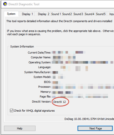
Fig. 3. Checking the DirectX version

Note:

The first time you use the DirectX diagnostic tool, you may be prompted to check for digital signatures on your drivers. It is recommended to select Yes to ensure that your drivers are signed by a publisher that has verified their authenticity.

Optimizing computer resource consumption for the rendering loop:

• OnTimer() or OnChartEvent() — for static scenes, call the Redraw() function only when data changes, not every tick;
• Level of Detail (LOD) — reduce the detail of objects as the camera moves away;
• Instancing - for multiple identical objects (clusters, markers), use one mesh with different transformation matrices.

The basic pipeline is ready. We created a canvas, set up a projection, defined objects with vertices and normals, applied transformations and lighting. The next step is to fill this framework with analytical content: transform optimization results into 3D surfaces, liquidity clusters into volumetric structures, and scenario models into interactive reports.

Visualizing complex data — surfaces, clusters, scenarios

Once the basic DX pipeline is set up, we have an empty space ready to visualize the data. The next task is to transform the numbers from the tester's report into geometric primitives understandable to the human eye. We move from raw matrices to visual landscapes.

Building a 3D optimization surface is probably the most useful way to use 3D in trading. The strategy tester produces a table where the rows are runs and the columns are parameters and metrics. Visualizing the optimization results in 3D turns this table into a terrain.

Simple visualization math: the X and Z axes become strategy parameters (e.g., moving average period and stop size), and the Y axis (height) becomes the target function (e.g., recovery factor, expected value). To build such a surface, we need to generate a triangle mesh (Mesh) based on the result array.

Construction algorithm:

• Data collection – go through the array of optimization results, select and structure the necessary data;
• Normalization - normalize parameter values to a common scale so that the graph does not look flattened;
• Vertex generation - for each data point we create the DXVertex vertex;
• Triangulation - connecting adjacent vertices with indices into triangles.

//+------------------------------------------------------------------+
//| example of creating a surface from a data array                  |
//+------------------------------------------------------------------+
void CreateOptimizationSurface(const double &data[],const int width,const int height)
  {
   DXVertex vertices[];
   uint indices[];
   int v_count = 0;
   int i_count = 0;
   
//--- allocate memory for vertices (width*height of points)
   ArrayResize(vertices,width*height);
   
   for(int y=0;y<height;y++)
     {
      for(int x=0;x<width;x++)
        {
         int idx=y*width+x;
         //--- X and Z are the coordinates of the parameters, Y is the value of the metric (profit)
         vertices[idx].position=DXVector3(x, data[idx], y); 
         vertices[idx].normal=DXVector3(0, 1, 0); // simplified normal
         vertices[idx].vcolor=ColorToVector4(ColorFromValue(data[idx])); // color depends on value
         vertices[idx].tcoord=DXVector2((float)x/width, (float)y/height);
        }
     }
   
//--- next, we form an array of indices for triangles and create an object using m_mesh.Create(...)
  }

On such a surface, "plateaus" are immediately visible — wide zones where the strategy operates relatively stably when parameters change. Conversely, narrow profit peaks (similar to needles) are clearly visible, which indicate overfitting. Visually cutting off such a "needle" is much easier than noticing it in a table of 1000 rows, given that multidimensional dependencies are poorly visible in tabular form.

Cluster analysis in space

Market data includes not only price and time, but also volume. In 2D, we usually draw a volume histogram at the bottom of the screen, but in 3D, volume becomes a full-fledged dimension. Instead of flat bars, we can use volume blocks (voxels) or cylinders, the height and thickness of which depend on trading volume or cluster density:

• X axis - Time;
• Z axis - Price;
• Y axis — Volume / Number of trades (voxel radius).

Liquidity visualization - using DXComputeSphere or custom meshes, you can draw large clusters of trades as spheres of varying sizes and transparency. Superimposed on each other, they create a cloud of liquidity, where the trader sees "voids" (zones where the price has moved quickly) and "clots" (support/resistance levels).

//--- setting color based on volume (heatmap effect)
//--- the larger the volume, the redder the color (from blue to red)
color cluster_color=ColorInterpolate(clrBlue,clrRed,volume_ratio);
m_cluster.MeshColorSet(ColorToVector4(cluster_color,0.7)); // 0.7 - transparency

Surface generation via DXComputeSurface()

For typical tasks of visualizing two-dimensional data (heat maps, optimization results, correlation matrices), the DirectX MQL5 library provides the DXComputeSurface() ready-made template function. The function is located in the DXUtils.mqh file.

Declaration:

//+------------------------------------------------------------------+
//| Surface                                                          |
//| TVertex must have                                                |
//| DXVector4 position, DXVector4 normal and DXVector2 tcoord members|
//+------------------------------------------------------------------+
template <typename TVertex>
bool DXComputeSurface(double &data[],uint data_width,uint data_height,double data_range,
                      const DXVector3 &from,const DXVector3 &to,DXVector2 &texture_size,
                      bool two_sided,bool use_normals,
                      TVertex &vertices[],uint &indices[])

Purpose:

Automatically generates vertices and indices for a 3D surface based on a 2D data array. The function frees the developer from the need to manually calculate coordinates, mesh triangulation, and normals.

Inputs:

Parameter	Type	Description
[in] data[]	double&	One-dimensional array of height values (optimization data, correlations, etc.)
[in] data_width	uint	Width of the original data matrix (number of columns)
[in] data_height	uint	Height of the original data matrix (number of rows)
[in] data_range	double	Scaling range for values along the Z axis (height)
[in] from	const DXVector3&	Coordinates of the lower left corner of the surface in 3D space
[in] to	const DXVector3&	Coordinates of the upper right corner of the surface in 3D space
[in] texture_size	DXVector2&	Texture coordinate size (for texture mapping or gradients)
[in] two_sided	bool	Double-sided rendering flag (useful for transparent surfaces)
[in] use_normals	bool	Normal calculation flag for correct lighting
[out] vertices[]	TVertex&	Output vertex array (filled by the function)
[out] indices[]	uint&	Output array of indices for triangulation (filled by the function)

TVertex type requirements - the TVertex template parameter should be a structure containing at least three fields:

struct MyVertex
  {
   DXVector4 position;  // vertex coordinates (x,y,z,w)
   DXVector4 normal;    // normal vector (nx,ny,nz,0)
   DXVector2 tcoord;    // texture coordinates (u,v)
   // additional fields as needed: color, binormal, etc.
  };

Returned value:

• true — the surface successfully generated;
• false — error (check array sizes and input data validity).

Sample use:

Let's say we have the results of strategy optimization in the form of a 20x20 matrix, where each value is the expected value of a trade. We want to visualize this data as a 3D surface.

//+------------------------------------------------------------------+
//| Generate optimization surface via DXComputeSurface               |
//+------------------------------------------------------------------+
void BuildOptimizationSurface(double &optimization_data[],uint width,uint height)
  {
//--- define the vertex type with an additional color field
   struct SVertex
     {
      DXVector4 position;
      DXVector4 normal;
      DXVector2 tcoord;
      DXColor   vcolor;  // vertex color for gradient
     };
   
   SVertex vertices[];
   uint    indices[];
   
//--- surface parameters
   DXVector3 from(-10.0,-5.0,0.0);   // lower left corner
   DXVector3 to(10.0,5.0,1.0);       // upper right corner
   DXVector2 texture_size(1.0,1.0);  // full coverage of texture coordinates
   double    data_range=2.0;         // height scaling
   
//--- generate geometry
   if(!DXComputeSurface(optimization_data,width,height,data_range,
                        from,to,texture_size,
                        false,true,  // one-sided, with normals
                        vertices,indices))
     {
      Print("surface generation error: ",GetLastError());
      return;
     }
   
//--- color the vertices by height (gradient: red → green)
   for(uint i=0;i<ArraySize(vertices);i++)
     {
      double t=MathMax(0.0,MathMin(1.0,vertices[i].position.z/data_range));
      vertices[i].vcolor=DXColor(1.0f-(float)t,(float)t,0.2f,1.0f);
     }
   
//--- create a mesh and add it to the scene
   if(!mesh.Create(canvas.DXDispatcher(),canvas.InputScene(),vertices,indices))
      Print("error creating mesh: ",GetLastError());
   
   mesh.DiffuseColorSet(DXColor(1.0f,1.0f,1.0f,1.0f));
   canvas.ObjectAdd(&mesh);
  }

DXComputeSurface() advantages:

• Development speed - no need to write triangulation and normal calculation cycles manually;
• Optimization - the internal implementation uses efficient mesh generation algorithms;
• Flexibility - the template vertex type allows adding any additional attributes (color, texture, custom data).

DXComputeSurface() limitations:

• Regular grids only - the function assumes that the data is a rectangular matrix. For irregular point clouds or arbitrary topology, manual generation will be required;
• Default interpolation - vertex heights are interpolated linearly between grid nodes. Pre-filtering of the data may be required to smooth jagged surfaces;
• Memory - the function allocates vertex and index arrays dynamically. When working with large matrices (e.g. 100x100 and larger), make sure to monitor memory consumption and surface rebuilding frequency.

Integration with interactive control:

Since DXComputeSurface() generates static geometry, dynamic updates (e.g. when changing optimization parameters in real time) require:

1. Save a reference to the CDXMesh object,
2. When data changes, call mesh.Shutdown() to free old buffers,
3. Re-call DXComputeSurface() and mesh.Create() with the new data,
4. Call RedrawScene() to display the changes.

For smooth animation, it is recommended to move heavy operations to the OnTimer handler, as is done in the DX_OptimizationSurface EA (see the description below). Using DXComputeSurface() in many typical cases reduces the amount of code by 30–40% when constructing typical surfaces, allowing us to focus on analytical logic rather than low-level graphics.

Scenario modeling and interactive reports

One of the advantages of DirectX in MQL5 is the ability to dynamically update the scene without reloading the indicator. This opens the way to modeling "what if?" scenarios. For example, the panel where you move the slider labeled "Volatility" or "Commission". The data[] array is recalculated in real time, and the VertexSet() vertex buffer update function dynamically changes the 3D surface.

//+------------------------------------------------------------------+
//| dynamic update example                                           |
//+------------------------------------------------------------------+
void OnSliderChange(const double new_vol)
  {
//--- recalculate the strategy metrics with the new volatility
   RecalculateStrategyMetrics(new_vol);
   
//--- update only the Y-coordinate of the vertices (height), without recreating the mesh
   for(int i=0;i<ArraySize(m_vertices);i++)
     {
      m_vertices[i].position.y=m_new_metrics[i];
      //--- recalculate normals for correct lighting
      m_vertices[i].normal=CalculateNormal(i); 
     }
   
//--- send updated data to video memory
   m_mesh.VertexSet(m_vertices);
   Redraw();
 }

This allows the trader to see the sustainability of the strategy - if a small change in volatility turns a profitable chart into a losing one, the strategy is unlikely to be viable over the long term.

Shaders as an analytical filter

MetaTrader 5 standard shaders are responsible for lighting (Phong model). But for analytics we need shaders that work with data. We can write a simple Pixel Shader that will act as a filter.

For example, you need to highlight on the 3D chart only those zones where the drawdown exceeds 20%, or where the profit factor is less than one:

//+------------------------------------------------------------------+
//| example of logic in HLSL shader                                  |
//+------------------------------------------------------------------+
float4 PS_Main(PS_INPUT input) : SV_TARGET
  {
//--- input.color contains the metric information encoded in the vertex
   float profit=input.color.r; 
   
//--- if the profit is below the threshold, make the object transparent
   if(profit<threshold)
      return float4(0.5,0.5,0.5,0.2); // gray and transparent
   else
      return float4(0.0,1.0,0.0,1.0); // bright green
  }

In the shader, we check the value of a vertex attribute (such as height or passed color) and, if it does not meet the criteria, we make the pixel transparent or gray. This approach allows us to remove "noise" from the graph, leaving only significant areas. This is important when analyzing large arrays of optimization data.

Interactivity - mouse, buttons and camera control

A static 3D image is beautiful, but it is of little use in trading if you cannot rotate, zoom, or filter it. The real benefit of DirectX in MQL5 comes when we get the opportunity to actively explore data. Let's look at how to bring a scene to life by linking mouse and keyboard events with camera math.

Event handling in MQL5 — bringing the canvas to life

By default, canvas (CDXCanvas) is just a raster image that does not respond to the cursor. To make it interact with the user, you need to subscribe to the chart events. This is done through the CHART_EVENT_MOUSE_... modifiers in the OnInit() function:

//+------------------------------------------------------------------+
//| subscribe to mouse events                                        |
//+------------------------------------------------------------------+
int OnInit()
  {
//--- enable receiving mouse events
   ChartSetInteger(0,CHART_EVENT_MOUSE_MOVE,1);
   ChartSetInteger(0,CHART_EVENT_MOUSE_WHEEL,1);
   
//--- timer for animation
   EventSetMillisecondTimer(16); 
   
   return(INIT_SUCCEEDED);
  }

After this, all cursor movements will be processed by the OnChartEvent() handler. The next task is to filter the required IDs (CHARTEVENT_MOUSE_MOVE, CHARTEVENT_MOUSE_WHEEL) and pass the coordinates to the rendering part of the code.

Remarks:

In OnDeinit(), be sure to disable these events (by calling ChartSetInteger(..., 0)), otherwise after deleting the indicator, the terminal will continue to generate them and create an extra load.

Camera control — orbit and zoom

The most commonly used way to interact with 3D graphics is to rotate around an object (orbit) and zoom in/out. In DirectX, this is achieved not by rotating the object itself, but by moving the camera on a sphere around the center of the scene.

Three interrelated methods are used to control the camera in CCanvas3D:

• ViewPositionSet() — set the location of the observer's eye (camera coordinates);
• ViewTargetSet() — set where the observer is looking (usually the center of the scene is 0,0,0);
• ViewUpDirectionSet() — set the direction of the top of the frame (so that the camera does not flip).

Implementation of rotation

Rotation is performed by moving the mouse cursor while holding down the left mouse button. To rotate the scene, we track the cursor movement delta: the difference between the current and previous position. We convert this delta into rotation angles around the X and Y axes.

//+------------------------------------------------------------------+
//| mouse movement event handler                                     |
//+------------------------------------------------------------------+
void OnMouseMove(int x, int y, uint flags)
  {
//--- check that the left mouse button is pressed
   if((flags&1)==1) 
     {
      //--- calculate the change in angles based on the mouse offset
      //--- divide by the coefficient (for example, 300.0f) for sensitivity
      m_camera_angles.y+=(x-m_mouse_x)/300.0f;
      m_camera_angles.x+=(y-m_mouse_y)/300.0f;
      //--- limit the vertical angle
      if(m_camera_angles.x<-DX_PI*0.49f)
         m_camera_angles.x=-DX_PI*0.49f;
      if(m_camera_angles.x>DX_PI*0.49f)
         m_camera_angles.x=DX_PI*0.49f;
      //--- recalculate the camera position
      UpdateCameraPosition();
      Redraw();
     }
//--- save the current coordinates for the next step
   m_mouse_x=x;
   m_mouse_y=y;
  }

In the UpdateCameraPosition() function, we use the DXMatrixRotationX and DXMatrixRotationY rotation matrices to rotate the camera's direction vector and update its position in space.

Zoom implementation

Rotating the mouse wheel changes the distance from the camera to the center of the scene (m_camera_distance).

//+------------------------------------------------------------------+
//| mouse wheel rotation event handler                               |
//+------------------------------------------------------------------+
void OnMouseWheel(double delta)
  {
//--- decrease or increase the distance
   m_camera_distance*=1.0-delta*0.001;
   
//--- limit the zoom to reasonable values
   if(m_camera_distance>50.0)
      m_camera_distance=50.0;
   if(m_camera_distance<3.0)
      m_camera_distance=3.0;

   UpdateCameraPosition();
   Redraw();
  }

UI panel on top of 3D scene

3D graphics are responsible for displaying data, but to control parameters we need standard and familiar MQL5 interface elements. To avoid reinventing the wheel, use the classes of the standard MQL5 control library (CAppDialog, CSlider, CComboBox etc.), which are drawn on top of or to the side of the graphic canvas. You can also use any other classes to build the interface.

When the slider value changes (for example, "Profit Threshold"), a function is called that updates the data in the vertex buffer or changes the shader variables, after which the Redraw() function is called. This allows us to create a full-fledged analytical tool. For example: on the left is an interactive 3D landscape displaying the optimization results, on the right is a control panel with filters.

Optimizing the interactive cycle

Interactivity should not significantly reduce the performance of the terminal and the computer as a whole. If you call the Redraw() function with each micro-movement of the mouse without holding down the button, the terminal interface will start to slow down.

Let's formulate the basic rules for optimizing interactivity:

• Call Redraw() only when necessary - call scene redraw only inside check blocks: if((flags & 1) == 1) (check when the button is pressed) or when changing UI parameters;
• Filtering out unnecessary events - if data for redrawing comes too often (for example, from ticks in the OnTick() handler), update the vertex buffer no more than 10-15 times per second;
• Asynchrony of heavy calculations - if changing a parameter requires recalculating thousands of vertices (for example, rebuilding the entire optimization surface), do it in the OnTimer() timer event handler or move it to a separate thread via DLL to avoid freezing the interface.

Test expert for validating 3D technologies

We will develop an EA implementing the described 3D technologies. The EA is a tool for three-dimensional visualization of analytical data in the MetaTrader 5 trading terminal. The main purpose is to transform the numerical results of trading strategy optimization into three-dimensional surfaces, allowing the trader and/or developer to quickly evaluate the quality and stability of the strategy.

The EA solves the following problems:

• Visualization of the optimization surface is a display of the dependence of the objective function (profit, expected value, Sharpe ratio) on two optimized strategy parameters in the form of a three-dimensional landscape.
• Strategy stability analysis – identifying "plateaus of stability" (areas with smooth changes in results) and "overfitting needles" (isolated peaks indicating overfitting to historical data).
• Interactive data exploration - providing the ability to rotate, zoom, and explore the surface in detail with a mouse.
• Mode comparison – switch between different display modes (e.g. profit and noise) to evaluate optimization quality.

Features:

3D visualization — the EA creates an interactive 3D canvas on the chart measuring 640×480 pixels, which displays a surface generated based on the analytical function. The surface is a 25x25 vertex mesh, triangulated for correct display.

Color coding — the following color scheme was applied:

• The top (maximum values) is a rich green color;
• Base (minimum values) - rich red color;
• Intermediate values are a smooth gradient with a transition through yellow-orange shades.

This coding allows us to confidently identify zones of maximum profit (green "hills") and zones of losses (red "troughs").

Camera control — full control of the viewpoint has been implemented:

• Rotation - holding down the left mouse button and moving the cursor rotates the camera around the center of the scene in a spherical orbit;
• Zooming - scrolling the mouse wheel zooms the camera in or out (distance from 5.0 to 40.0 units);
• Limitations - the vertical angle is limited to ±0.9×π/2 to prevent the camera from flipping.

Interactive control

There is a mode switching button on the canvas:

• Profit mode - displays a smooth Gaussian curve surface (simulating a stable strategy);
• Noise mode - displays the surface with added random noise (simulating an over-optimized strategy).

When switching modes, the button text is automatically updated.

Lighting and materials

To create a realistic volumetric image, a Phong lighting model with three components was used:

• Directional light source - yellow color (1.0, 0.95, 0.8), direction (0.5, -0.8, 0.3);
• Ambient lighting - gray color (0.55, 0.55, 0.55) with increased intensity for better visibility of shadow areas;
• Diffuse material - white color (1.0, 1.0, 1.0, 1.0) for correct mixing with vertex colors.

Implementation features

Asynchronous event handling:

• Reaction to mouse cursor movements and wheel rotation - the program receives the OnChartEvent() function call and immediately handles it (the orientation of the 3D model, its dimensions, etc. are changed). There are no complex calculations involved.
• Reaction to pressing the mode switch button - the program receives the OnChartEvent() function call and sets the need_rebuild flag. The BuildSurface() function responsible for destroying the old mesh, generating a new 3D surface and rendering is called inside the OnTimer() handler function, which checks the state of the need_rebuild flag every 50ms.

This approach ensures that even if recalculating the 3D model takes up CPU resources, the terminal chart and controls remain fully responsive.

The MQL5\Include\Canvas\DX\DXMath.mqh library is used to correctly calculate lighting and camera orientation:

• Normals - for each vertex of the surface, the normal vector is calculated using the DXVec3Cross() vector product function. This is necessary so that the surface has volume and reacts to the light source, creating realistic shadows and highlights.
• Camera - the observer's position is calculated using spherical coordinates, which allows for intuitive rotation around an object ("orbit") without the effect of camera flipping, limiting the vertical angle.

The full code of the EA is contained in the DX_OptimizationSurface.mq5 file attached to the article.

Examples of the EA's work in different modes are shown in the figures below:

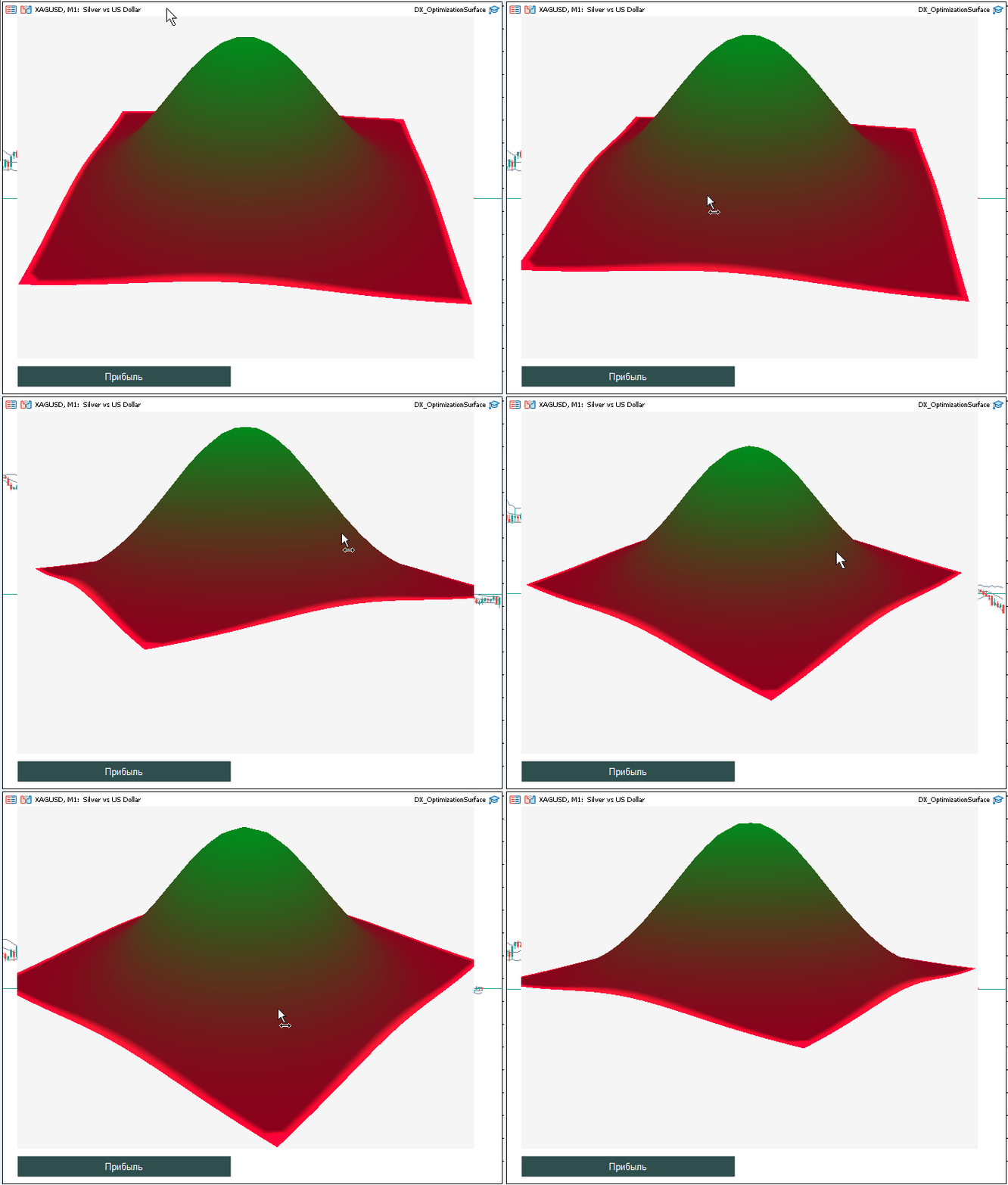
Fig. 4. Profit mode

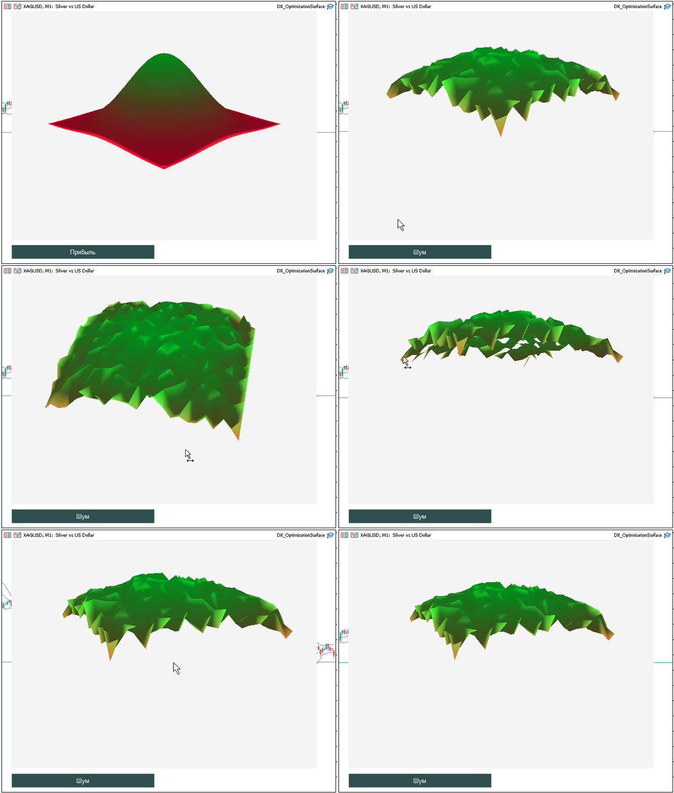
Fig. 5. Noise mode

Now we have a full set of tools: we can build a scene, fill it with optimization data, and give the user the ability to explore this data by rotating and zooming. But before rushing to implement 3D everywhere possible, let's first look at where this technology is unnecessary and where it is better to stick with conventional graphs.

When is it better to stick with regular graphs?

A tool is only useful when it solves a problem faster and more accurately than its predecessor. We have explored the DX pipeline architecture, learned how to generate surfaces, and control the camera. However, in trading, one must distinguish between useful analytical visualization and the chaos of visual noise. Integrating 3D graphics into MetaTrader 5 is not an end in itself, but a way to solve problems. Let's consider cases where abandoning 3D in favor of classic 2D will be technically and economically justified.

Data dimensionality rule

Let's formulate a rule for the necessity of 3D visualization: the third dimension must carry unique information:

• 3D is useless - if you are trying to display a time series (Price/Time) in 3D space. Adding a Z axis that duplicates price or time will only complicate perception, forcing the trader to rotate the scene to see the regular trend line.
• 3D is necessary when analyzing optimization results. Here we have two independent inputs (for example, the moving average period and the stop size) and one output metric (profit or profit factor). Without a 3D surface, we will see only a set of points. 3D allows us to see the relationship between two variables and the outcome.

If your dataset boils down to a pair of coordinates, a regular 2D graph (DRAW_LINE, DRAW_HISTOGRAM) will be more efficient.

Hardware limitations and VPS

3D graphics in MQL5 are based on DirectX 11. This requires Shader Model 5.0 support and a certain level of CPU/GPU performance.

Most professional developers run their EAs on virtual private servers (VPS). Many standard VPS configurations do not have powerful graphics cards or DirectX hardware acceleration. In such environments, calling CreateBitmapLabel() may cause an EA error and/or crash.

Therefore, if your program is designed to run in "blind" mode, i.e. without graphics, or on a cheap server, the 3D module should be disabled or replaced with logging to a file/database. 2D graphics can be easily rendered by the CPU even without a video card.

Perception speed — 3D Surface against Heat Map

One of the main alternatives to a 3D surface is a two-dimensional heat map (HeatMap). The fundamental differences between them are as follows:

• 3D - shows height (Z) as physical elevation. Requires rotation to accurately analyze all sides and hidden slopes.
• HeatMap — shows the (Z) value as the color of a cell on the (X, Y) plane.

If the goal is to quickly find the maximum optimization (the greenest zone), the HeatMap in the standard indicator will work faster and require less code.

Interactivity vs Monitoring

Interactive 3D scenes (like our DX_OptimizationSurface EA) require active human participation. You have to hover your mouse, hold down the button, and rotate.

If the purpose of the chart is monitoring (background tracking of the situation), then interactive 3D graphics can be distracting and slow down the process.

If the goal is a presentation or in-depth analysis before launching a strategy, then 3D is indispensable.

Conclusion: 

Use 3D only when the volume of data or its structure makes analysis in 2D impossible. If your goal is to quickly find the maximum in an optimization table, a heat map will do the job better. 3D is needed where you need to see the form of the relationship, and not just the value.

In other cases, standard MQL5 classes (CCanvas for 2D or graphical objects) will be a simpler solution.

Conclusion

We have gone from theoretically justifying the need for 3D graphics to creating a fully-fledged interactive EA. The DX_OptimizationSurface EA demonstrates that MetaTrader 5 is not just a terminal for order execution, but a powerful platform for visual data analysis.

Key findings:

• Cognitive efficiency – 3D visualization allows us to transform endless arrays of numbers into visual landscapes. This reduces the cognitive load on the trader, allowing them to visually distinguish stable profit plateaus from dangerous overfitting needles.
• Technological accessibility – built-in DirectX 11 support and native CCanvas3D and CDXMesh classes give developers the tools to solve trading problems. There is no need to write C++ code or include external libraries - everything is already inside MQL5. All that remains is to take advantage of it.
• The importance of architecture — as we saw, integrating graphics requires careful attention to resource lifecycles and asynchronicity. Moving computational operations to a timer and properly clearing memory is a guarantee that there will be no problems with terminal performance.

Visualization is a lens, not a decoration. It should answer a specific analytical question.

We created this tool not for the sake of external effect, but to speed up decision-making. If 3D graphics help you quickly understand the behavior of a strategy and filter out unviable options, then it has served its purpose. If it is just a distraction, feel free to return to proven 2D methods. A tool is valuable not because of how it looks, but because of the decisions it helps accelerate.

Next steps - for those who want to delve deeper into the topic, we recommend the following:

• Exploring the DXMath library for working with quaternions and complex transformations.
• Developing custom shaders (HLSL) to create unique rendering effects.
• Integrating with Python via MetaTrader 5 for pre-processing data before visualizing it in the terminal.

MetaTrader 5 provides the technological foundation. The analytical tools you build on it depend only on your imagination and the need to search for "pearls" in endless market data.

Recommended resources for learning how to work with DirectX in MetaTrader 5:

• MetaEditor DirectX help,
• How to create 3D graphics using DirectX in MetaTrader 5,
• DirectX Tutorial (Part I): Drawing the first triangle,
• Visualize a Strategy in the MetaTrader 5 Tester.

List of files attached to the article:

File Name	Description
DX_OptimizationSurface.mq5	A file containing the code of a test EA with interactive 3D visualization