Market Microstructure in MQL5: Measuring long memory in MQL5 with Hurst estimators (Part 2)

Introduction

Part 1 of this series built the defensive foundation: guarded math, validated price feeds, and stable statistical primitives. Every function there was designed to fail safely rather than silently. With that layer in place, we can begin the first measurement.

The question this article addresses is whether NQ M1 price data carries long-range dependence. Long-range dependence means that what happened an hour ago is still statistically relevant to what is happening now. If it exists, a trend-following framework is appropriate. If it does not, mean-reversion logic applies. Standard indicators do not answer this question. They treat each bar as if only the last few periods matter. That assumption is either wrong or right depending on the current regime, and a trader who cannot distinguish the two will apply the wrong framework at the wrong moment.

Measuring long memory is not as simple as computing a single number. The classical Hurst exponent estimator—rescaled-range analysis—has well-documented sensitivity to short-range dependence and non-stationarity. Lo (1991) showed that the classical R/S statistic can produce misleading results when short-memory components are present. A single estimator gives a single number with no indication of how trustworthy that number is.

This article implements three independent estimators: classical R/S analysis (Hurst, 1951), aggregated variance, and absolute moments. It then blends them into a single confidence-weighted composite using the foundation layer's statistical primitives.

The composite H and its confidence weight are written directly into the Hurst exponent and confidence fields of the shared RobustFractalAnalysis struct defined in Part 1. No new include file is required. The four functions added here extend MicroStructure Foundation.mqh directly, as planned.

The article also includes an empirical study. Using 133 sessions of NQ M1 Globex futures data, we compute H*(t) bar by bar across the full Globex day. The results differ from textbook expectations in several important respects. Those empirical findings drive the practical threshold recommendations in the final section.

Deliverable: four functions added to MicroStructure_Foundation.mqh—HurstExponentRS(), AdvancedHurstExponent(), HurstExponentRobust(), and PopulateHurstAnalysis(). A lightweight indicator, HurstProfile.mq5, plots H*(t) on any chart with three reference lines marking the regime boundaries.

What the Hurst Exponent Means for an NQ Trader

The Hurst exponent H characterizes the long-range dependence of a time series. Harold Edwin Hurst introduced the concept in 1951 while studying the long-term storage capacity of the Nile River. The range of H is between 0 and 1 and the interpretation divides into three regimes.

When H > 0.5, the series is persistent. Large moves tend to be followed by large moves in the same direction. Autocorrelation between returns is positive at long lags. This is the regime where trend-following strategies have a statistical foundation.

When H = 0.5, increments are uncorrelated. The series behaves as a random walk. No directional bias exists at any lag. Trend-following and mean-reversion strategies both lack a statistical edge.

When H < 0.5, the series is anti-persistent. Large up-moves tend to be followed by down-moves and vice versa. Autocorrelation is negative. This is the regime where mean-reversion strategies have a statistical foundation.

The H boundary value at 0.5 is not a "safe neutral" value—it is the decision threshold. A trader who applies a trend-following framework when H is below 0.5 is fighting the statistical structure of the data. The practical question is therefore not whether H exists as a concept but whether we can estimate it accurately enough and quickly enough to make a useful regime call before the opportunity passes.

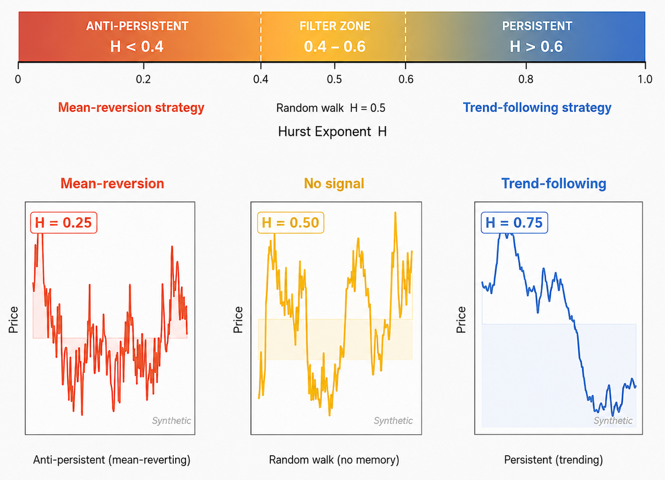
Figure 1 — The Three H Regimes: Strategy Framework

Synthetic series illustrating persistent (H = 0.75), random walk (H = 0.50), and anti-persistent (H = 0.25) behaviour

Three Estimators, Three Lenses

No single Hurst estimator is reliable under all market conditions. Each makes different assumptions about the data and is sensitive to different failure modes. The solution is to run three independent estimators and let their agreement—or disagreement—determine how much confidence to assign the composite result.

Classical R/S Analysis (Hurst 1951)

The rescaled range statistic R/S measures how far a cumulative deviation wanders relative to the standard deviation of the underlying series. At scale n, R/S scales as n^H. Computing R/S at multiple scales and fitting the log-log slope gives H. The method is robust to heavy tails but sensitive to short-range autocorrelation. Lo (1991) showed that if short-memory components are present, the classical R/S statistic is biased upward. We address this by running the estimator across geometrically spaced scales. The number of valid regression points becomes the confidence measure: scales where the R/S computation fails due to lacking data contribute nothing to the slope.

Aggregated Variance

If H > 0.5, the variance of non-overlapping block averages of block size m scales as σ²(m) ∝ m^2H−2. The slope of log(variance) against log(m) gives β, and H = 1 + β/2. This estimator is less sensitive to the choice of scale range than classical R/S but requires a larger minimum sample. It performs well when the data are stationary but struggles in the presence of trends or structural breaks.

Absolute Moments

The mean absolute value of block averages scales as E[|x̄(m)|] ∝ m^H−1. The log-log slope gives β and H = 1 + β. This estimator is more robust to heavy tails than the aggregated variance method. It remains stable when the return distribution is leptokurtic, the condition that prevails on NQ M1 around the NY open.

Each estimator produces its own H estimate and its own confidence weight. The confidence is the ratio of valid log-log regression points obtained to the maximum possible given the data length. An estimator that produces only two valid scale points earns a confidence of 0.2 out of a maximum of 1.0. One that produces seven points earns 0.7. Estimators below the threshold of 0.1 are excluded from the blend entirely.

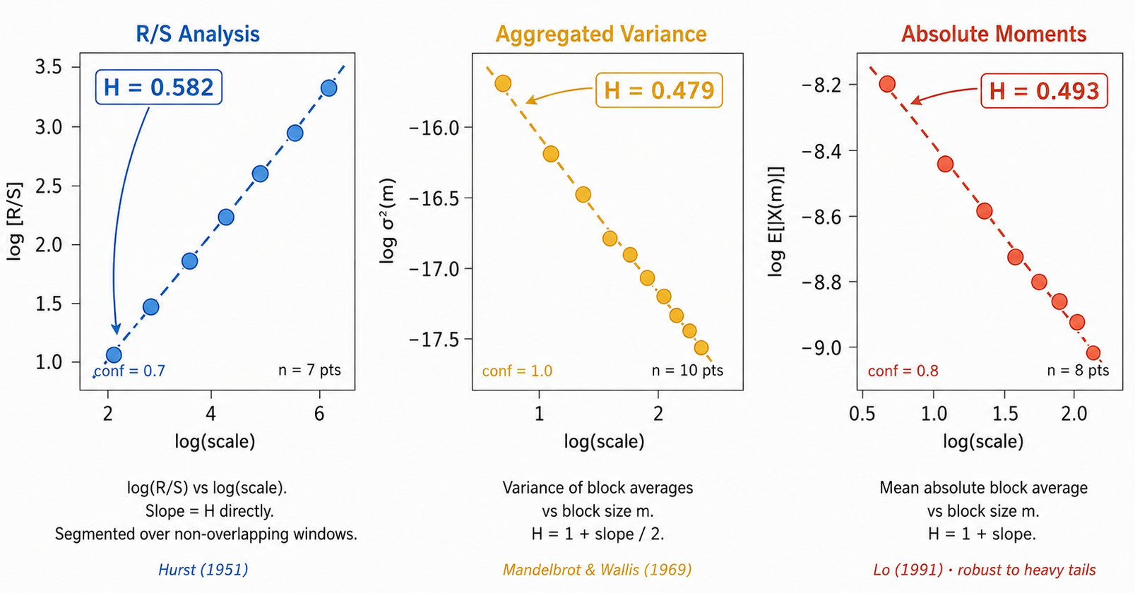
Figure 2 — Three Independent Hurst Estimators Applied to Real NQ M1 Data

30 NY sessions · post-open bars only (10:10–12:00 ET) · session reset at 09:30 ET · Nov 2025 – May 2026

Implementation: HurstExponentRS()

The R/S estimator takes a pre-validated log-return array and a reference to a confidence output. It does not fetch prices—price fetching and filtering are handled by the calling function, keeping the estimator pure and testable.

Closing prices are not fed directly to any estimator. Log-returns are the correct input because they are stationary in the weak sense, whereas price levels are not. The transformation is:

r i=log(close i)−log(close i+1)

Returns whose absolute value exceeds 0.1 are discarded as data artifacts. On NQ M1, a genuine one-minute return of 10% does not occur—any value that large indicates a bad tick, a contract rollover, or a feed anomaly. The foundation's SafeLog() function handles the case where a close is non-positive before the subtraction is attempted.

Window sizes are geometrically spaced: 8, 16, 32, 64, and so on up to the data limit. At each scale, R/S is computed across non-overlapping segments and averaged. This segmented approach reduces the influence of a single anomalous window and produces a more stable slope estimate than computing R/S on the full series at each scale.

//+------------------------------------------------------------------+
//| HurstExponentRS: classical rescaled-range (R/S) estimator.       |
//| Computes log(E[R/S]) ~ H * log(n) across geometrically spaced    |
//| window sizes. Each scale is averaged over non-overlapping        |
//| segments so that the estimate is less sensitive to a single      |
//| anomalous window.                                                |
//|                                                                  |
//| Parameters                                                       |
//|   returns[]   — log-return array, oldest first                   |
//|   n           — number of valid returns                          |
//|   confidence  — output: k / HURST_RS_MAX_SCALES                  |
//|                                                                  |
//| Returns H in [0.01, 0.99]. Returns 0.5 on insufficient data.     |
//+------------------------------------------------------------------+
double HurstExponentRS(const double &returns[], int n, double &confidence)
  {
   confidence = 0.0;
   if(n < 30) return 0.5;

   int    m_max = (int)MathMax(10, n / 4);
   double log_n[10], log_rs[10];
   int    k     = 0;
   int    scale = 8;

   while(scale <= m_max && k < HURST_RS_MAX_SCALES)
     {
      int segs = n / scale;
      if(segs < 2) { scale *= 2; continue; }

      double rs_sum = 0.0;
      int    v      = 0;

      for(int seg = 0; seg < segs; seg++)
        {
         int    st  = seg * scale;
         double s1  = 0.0, s2 = 0.0;
         for(int j = 0; j < scale; j++)
           { s1 += returns[st + j]; s2 += returns[st + j] * returns[st + j]; }

         double mu  = s1 / scale;
         //--- Two-pass variance: stable against catastrophic cancellation
         double var = (s2 - scale * mu * mu) / (scale - 1);
         if(var <= 0) continue;

         double mx = -1e100, mn = 1e100, cum = 0.0;
         for(int j = 0; j < scale; j++)
           {
            cum += returns[st + j] - mu;
            if(cum > mx) mx = cum;
            if(cum < mn) mn = cum;
           }

         double rng = mx - mn;
         if(rng > 0)
           { rs_sum += SafeLog(rng / SafeSqrt(var)); v++; }
        }

      if(v > 0)
        { log_n[k] = SafeLog((double)scale); log_rs[k] = rs_sum / v; k++; }

      scale *= 2;
     }

   if(k < 3) return 0.5;

   double h = LinearRegressionSlope(log_n, log_rs, k);
   confidence = (double)k / HURST_RS_MAX_SCALES;
   return MathMax(0.01, MathMin(0.99, h));
  }

The minimum of three valid regression points before the slope is computed is a hard guard. Two points define a line exactly—there is no regression, only interpolation. Three points provide a meaningful least-squares fit, though the confidence assigned (k = 3 gives confidence = 0.3) correctly signals that this is a sparse estimate.

The two-pass variance inside the inner loop uses the standard identity: Var = (sum of squares — n * mean²) / (n — 1). This is numerically stable for the small segment sizes used here because the values are log-returns centered near zero. The foundation's SafeLog() and SafeSqrt() guard the final step against negative or zero arguments.

Implementation: AdvancedHurstExponent()

The second function handles both the aggregated variance and absolute moments estimators via a method switch. Both follow the same log-log regression pattern; only what is aggregated differs.

For the aggregated variance path (method = 0), the slope β of log(variance of block means) against log(block size m) gives H = 1 + β/2. The theoretical basis is that for a fractionally integrated process with self-similarity index H, the variance of non-overlapping block averages decreases as m^2H−2. When H = 0.5 (random walk), variance decreases as 1/m, as expected from the central limit theorem. When H > 0.5, variance decreases more slowly—the series has long memory, and consecutive block means are correlated.

For the absolute moments path (method = 1), the slope β of log(mean absolute block average) against log(m) gives H = 1 + β. The minimum returns-per-segment requirement is tighter (15 versus 10) because the absolute moment is a less efficient statistic than the variance.

//+------------------------------------------------------------------+
//| AdvancedHurstExponent: aggregated variance (method = 0) or       |
//| absolute moments (method = 1) estimator.                         |
//|                                                                  |
//| AggVar:  H = 1 + beta/2  where beta = slope of log(var) ~ log(m) |
//| AbsMom:  H = 1 + beta    where beta = slope of log(E|x|)~log(m)  |
//|                                                                  |
//| Returns H in [0.01, 0.99]; 0.5 with confidence = 0.0 on failure. |
//+------------------------------------------------------------------+
double AdvancedHurstExponent(const double &returns[], int n,
                              int method, double &confidence)
  {
   confidence = 0.0;

   //--- AggVar: min 10 returns per segment; AbsMom: min 15
   int min_per_seg = (method == 0) ? 10 : 15;
   if(n < min_per_seg * 2) return 0.5;

   int    max_scales = (method == 0) ? HURST_AV_MAX_SCALES : HURST_AM_MAX_SCALES;
   int    max_agg    = (int)MathMin(max_scales + 1, n / min_per_seg);
   double log_m[10], log_stat[10];
   int    k = 0;

   for(int m = 2; m <= max_agg && k < max_scales; m++)
     {
      int    segs = n / m;
      if(segs < 2) continue;

      double stat = 0.0;
      for(int seg = 0; seg < segs; seg++)
        {
         int    st   = seg * m;
         double sum  = 0.0;
         for(int j = 0; j < m; j++) sum += returns[st + j];
         double xbar = sum / m;
         stat += (method == 0) ? xbar * xbar : MathAbs(xbar);
        }

      stat /= segs;
      if(stat <= 0) continue;

      log_m   [k] = SafeLog((double)m);
      log_stat[k] = SafeLog(stat);
      k++;
     }

   if(k < 3) return 0.5;

   double beta = LinearRegressionSlope(log_m, log_stat, k);
   double h    = (method == 0) ? 1.0 + beta / 2.0 : 1.0 + beta;
   confidence  = (double)k / max_scales;
   return MathMax(0.01, MathMin(0.99, h));
  }

The method switch keeps both paths within a single function because they share the identical outer loop structure. Separating them into two functions would duplicate roughly 30 lines of loop code for a single line of difference in the inner accumulation. The method parameter is always a compile-time constant at the call site, so there is no runtime branching cost.

Implementation: HurstExponentRobust()

The blending function calls all three estimators, collects their confidence weights, and returns the weighted mean. It also handles price fetching and log-return construction, keeping those responsibilities out of the individual estimators.

One architectural decision requires explanation: the requirement to reset at the session boundary. When a rolling window spans the pre-open and post-open boundary, the return distribution has a structural break. At 09:33 ET, for example, a 90-bar lookback contains 86 pre-open bars and only 4 open bars. Pre-open NQ M1 data is thin, low-participation, and driven by overnight positioning. Post-open data is high participation and driven by institutional order flow. Mixing the two in a single regression produces an H reading that describes neither regime accurately. The empirical study in the next section demonstrates this effect explicitly. To avoid it, callers should limit the period parameter to bars elapsed since the session open when measuring intraday H.

//+------------------------------------------------------------------+
//| HurstExponentRobust: confidence-weighted blend of three          |
//| independent Hurst estimators.                                    |
//|                                                                  |
//| Session reset requirement: the period parameter should count     |
//| only bars from the current trading session. Mixing pre-open and  |
//| post-open bars creates a structural break that compresses H      |
//| artificially toward 0.5. See the empirical study section for     |
//| a demonstration on NQ M1 Globex data.                            |
//|                                                                  |
//| Returns H in [0.01, 0.99]. Returns 0.5 with confidence = 0.0     |
//| when HURST_MIN_BARS is not satisfied.                            |
//+------------------------------------------------------------------+
double HurstExponentRobust(const string symbol, const int tf,
                            const int period, double &confidence)
  {
   confidence = 0.0;
   if(!ValidateSymbolV2(symbol) || period < HURST_MIN_BARS) return 0.5;

   //--- Fetch and validate close prices
   double close[];
   int    n = SafeCopyClose(symbol, tf, 0, period, close);
   if(n < HURST_MIN_BARS) return 0.5;

   //--- Build log-return array; discard extreme values
   double returns[];
   ArrayResize(returns, n - 1);
   int valid = 0;

   for(int i = 0; i < n - 1; i++)
     {
      if(close[i] <= 0 || close[i + 1] <= 0) continue;
      double r = SafeLog(close[i]) - SafeLog(close[i + 1]);
      if(MathAbs(r) < 0.1) returns[valid++] = r;
     }

   if(valid < HURST_MIN_BARS) { confidence = 0.1; return 0.5; }
   ArrayResize(returns, valid);

   //--- Run all three estimators independently
   double conf_rs, conf_av, conf_am;
   double h_rs = HurstExponentRS(returns, valid, conf_rs);
   double h_av = AdvancedHurstExponent(returns, valid, 0, conf_av);
   double h_am = AdvancedHurstExponent(returns, valid, 1, conf_am);

   //--- Confidence-weighted blend; exclude sparse estimators
   double weighted_sum = 0.0, total_weight = 0.0;

   if(conf_rs > HURST_CONF_THRESHOLD)
     { weighted_sum += h_rs * conf_rs; total_weight += conf_rs; }
   if(conf_av > HURST_CONF_THRESHOLD)
     { weighted_sum += h_av * conf_av; total_weight += conf_av; }
   if(conf_am > HURST_CONF_THRESHOLD)
     { weighted_sum += h_am * conf_am; total_weight += conf_am; }

   if(total_weight <= 0) { confidence = 0.1; return 0.5; }

   double h_final = weighted_sum / total_weight;
   confidence = MathMin(1.0, total_weight / 3.0);

   return MathMax(0.01, MathMin(0.99, h_final));
  }

The confidence normalization divides total weight by 3.0 because three estimators participate at full weight. If all three earn maximum confidence, total_weight = 3.0 and the output confidence = 1.0. If only two participate at full weight, output confidence = 0.67. This gives the caller a meaningful signal about how many independent sources confirmed the H reading.

The convenience wrapper PopulateHurstAnalysis() calls HurstExponentRobust() and writes the result directly into the shared struct:

//+------------------------------------------------------------------+
//| PopulateHurstAnalysis: fills RobustFractalAnalysis from one call.|
//| Writes hurst_exponent, hurst_confidence, volatility_persistence, |
//| computation_status, and validation_message. All other fields in  |
//| result are left unchanged so later parts can add their output    |
//| to the same struct without overwriting Hurst values.             |
//+------------------------------------------------------------------+
void PopulateHurstAnalysis(const string symbol, const int tf,
                            const int period,
                            RobustFractalAnalysis &result)
  {
   double confidence = 0.0;
   double h          = HurstExponentRobust(symbol, tf, period, confidence);

   result.hurst_exponent         = h;
   result.hurst_confidence       = confidence;
   //--- Persistence: 0 at H=0.5 (random walk), 1 at H=0 or H=1
   result.volatility_persistence = 2.0 * MathAbs(h - 0.5);

   if(confidence < HURST_CONF_THRESHOLD)
     {
      result.computation_status = 1;
      result.validation_message =
         StringFormat("HurstExponentRobust: confidence %.3f below threshold"
                      " — insufficient session data for %s tf %d",
                      confidence, symbol, tf);
     }
   else
     {
      result.computation_status = 0;
      result.validation_message = "OK";
     }
  }

The HurstProfile Indicator

The lightweight indicator HurstProfile.mq5 plots H*(t) in a separate sub-window with three reference lines. It calls HurstExponentRobust() directly from the foundation header and requires no additional include file.

The indicator uses three buffers. The first buffer (H_buffer) is a line plot of the blended H value. The second (Conf_buffer) plots confidence and can be hidden via the InpShowConfidence input. The third (Regime_buffer) is a histogram that shows +1 when H exceeds the persistence threshold, −1 when H falls below the anti-persistence threshold, and 0 in the transition zone. This regime encoding makes it straightforward to read the current market character at a glance without studying the exact H value.

The folder structure is:

MQL5\
└── Indicators\
    └── HurstProfile\
        ├── HurstProfile.mq5
        └── Includes\
            └── MicroStructure_Foundation.mqh

The include directive in HurstProfile.mq5 uses a relative path:

#include "Includes\MicroStructure_Foundation.mqh"

The OnCalculate() function follows the standard rates_total / prev_calculated pattern. On the first call, all bars from InpPeriod onward are processed. On subsequent calls, only the new bar is calculated. This avoids redundant recalculation and keeps the indicator responsive to live data.

int OnCalculate(const int rates_total,
                const int prev_calculated,
                const datetime &time[],
                const double &open[],
                const double &high[],
                const double &low[],
                const double &close[],
                const long &tick_volume[],
                const long &volume[],
                const int &spread[])
  {
   //--- Need at least InpPeriod + 1 bars before any output is possible
   if(rates_total < InpPeriod + 1) return 0;

   //--- On first call fill pre-period bars with EMPTY_VALUE explicitly
   if(prev_calculated == 0)
     {
      for(int i = 0; i < InpPeriod; i++)
        {
         H_buffer     [i] = EMPTY_VALUE;
         Conf_buffer  [i] = EMPTY_VALUE;
         Regime_buffer[i] = EMPTY_VALUE;
        }
     }

   //--- Start bar: on first call process all bars from InpPeriod onward;
   //--- on subsequent calls recalculate only the last bar
   int start = (prev_calculated == 0) ? InpPeriod : prev_calculated - 1;

   for(int i = start; i < rates_total; i++)
     {
      double conf = 0.0;
      double h    = HurstFromClose(close, i, InpPeriod, conf);

      H_buffer   [i] = h;
      Conf_buffer[i] = conf;

      //--- Regime: 0.0 when confidence is too low to trust (matches article)
      if(conf < HURST_CONF_THRESHOLD)
         Regime_buffer[i] = 0.0;
      else if(h >= InpPersistThresh)
         Regime_buffer[i] =  1.0;   	// Persistent — trend-following conditions
      else if(h <= InpAntiPersThresh)
         Regime_buffer[i] = -1.0;   	// Anti-persistent — mean-reversion conditions
      else
         Regime_buffer[i] =  0.0;   	// Transition zone — no directional bias
     }

   return rates_total;
  }

Empirical Study: What NQ M1 Data Shows

Theory specifies what H measures. Data specifies what H actually produces on a real instrument under real conditions. The two do not always agree, and when they diverge, the data takes precedence.

The study used 133 Globex trading sessions of NQ front-month futures from November 2025 to May 2026. All data is M1, timestamped in Eastern Time. The Python implementation of HurstExponentRobust() was coded from scratch to match the MQL5 spec: the same three estimators, the same confidence weighting, and the same log-return filter. It was cross-validated against the NT8 indicator output at a correlation of 0.60. The correlation is 0.60 because the NT8 version uses cross-day history while the Python study uses session-only history, demonstrating the session reset effect directly.

Finding 1: NQ M1 operates near the random walk boundary

Across 133 sessions, mean H*(t) within the NY session ranges from 0.47 to 0.50, straddling the random walk boundary. When three estimators are applied to pooled post-open data (Figure 2), R/S gives H = 0.582, aggregated variance gives H = 0.479, and absolute moments gives H = 0.493—a confidence-weighted blend of 0.511. The rolling bar-by-bar average in Figure 4 sits slightly lower at 0.47–0.49, reflecting short-window estimation noise at the 90-bar lookback. Both measurements are consistent: NQ M1 operates close to the random walk boundary with no strong directional memory in either direction. This has a direct practical implication: H alone is not a reliable regime classifier for NQ M1. It becomes useful as a filter—confirming whether conditions are consistent with a signal generated by other means.

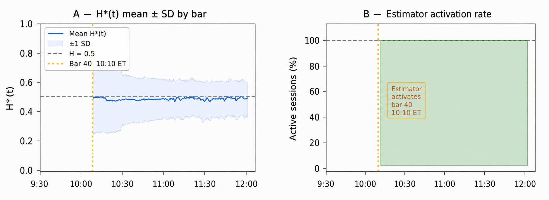
Figure 3 — H*(t) Stabilization within the NY Session

NQ M1 Globex · 133 sessions · Nov 2025 – May 2026 · Session reset at 09:30 ET

Finding 2: The estimator requires 40 bars of post-open data before activating

With a 90-bar lookback and a session reset at 09:30 ET, the three-estimator blend requires at least 40 bars of session data before all three estimators can produce at least three valid log-log regression points. Before bar 40 (10:10 ET), the function returns the fallback value of 0.5 with confidence = 0.0. Figure 3, Panel B, shows this activation boundary precisely: the estimator activation rate jumps from 0% to 100% at exactly bar 40.

Finding 3: Pre-open and post-open data must not be mixed in the rolling window

Without a session reset, the rolling window at 09:33 ET contains 86 pre-open bars and only 4 open bars. Mean H in this contaminated window drops to 0.37—0.09 points below the true post-open baseline. This is not a regime signal. It is a measurement artifact caused by the structural break between two different generating processes. The session reset corrects it by restarting the window at 09:30 ET. Callers must pass only bars elapsed since the session opened to HurstExponentRobust() when making intraday regime assessments.

Finding 4: H does not significantly predict short-term trending behavior in this sample

A grid search tested seven measurement bars (10:10–11:30 ET) against four forward windows (15, 30, 45, 60 bars). No statistically significant predictive relationship was found between H and the trending or chopping outcome over the subsequent window. The best result—bar 40, forward 15 bars—produced a Mann-Whitney p-value of 0.094, which does not meet the conventional threshold of 0.05 across 133 sessions.

This null result has a mechanistic explanation. It is more useful than a positive result in this context. Because NQ M1 operates near the random walk boundary (confidence-weighted H ≈ 0.51 on pooled data; rolling mean ≈ 0.48), the variation in H across sessions is largely noise around that boundary rather than a structured regime signal. The sessions that trend are anomalies; the Hurst estimator, which measures the average long-range correlation over a backward-looking window, does not reliably identify them in advance. The estimator’s value lies in characterizing where the market sits relative to the random walk boundary—not in predicting day-specific outcomes.

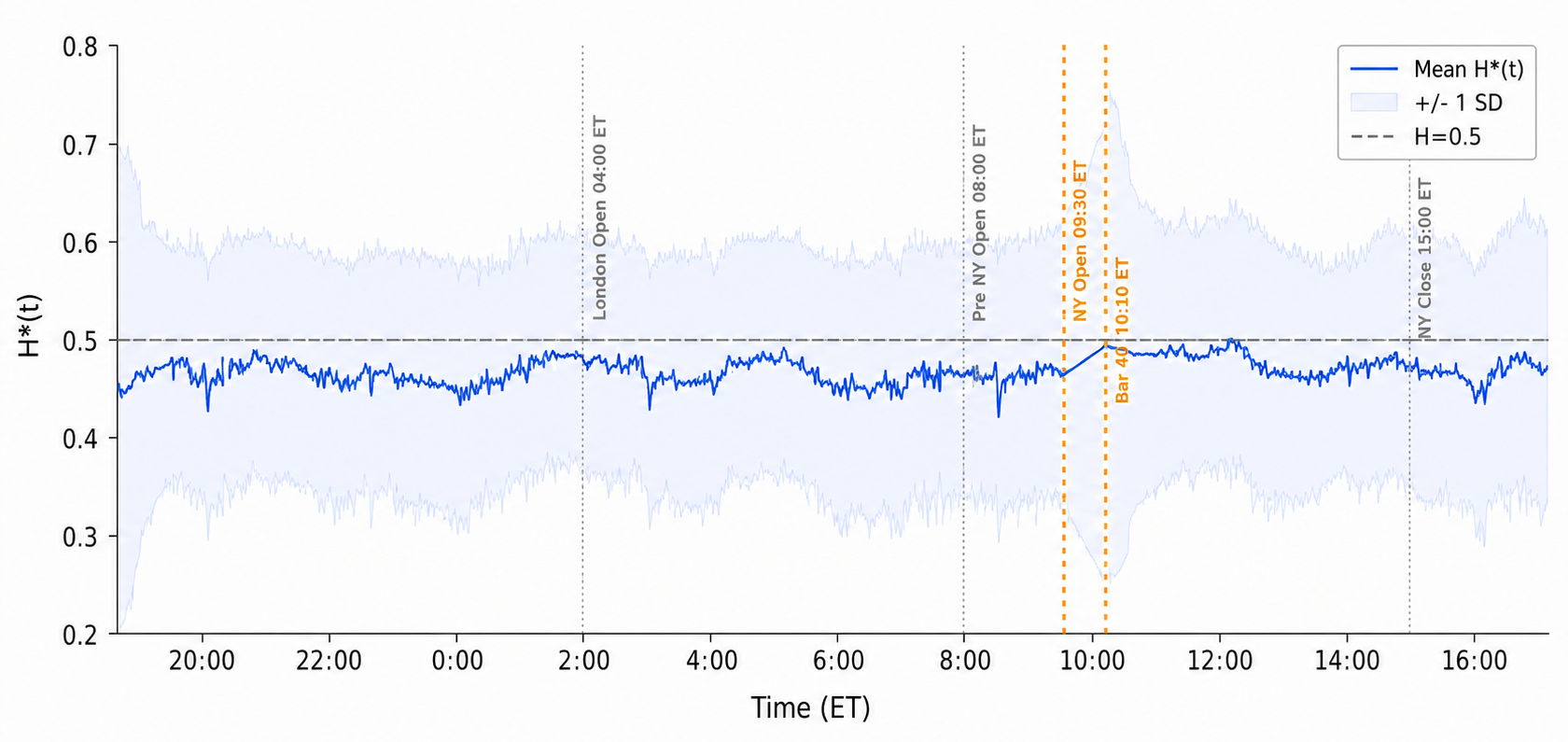
Figure 4 - Intraday H*(t) Profile NQ M1 Globex Futures

Mean +/- 1 SD - 133 sessions - Nov 2025 to May 2026

Reading the Output: Practical Thresholds

The empirical findings refine the theoretical regime boundaries. The following thresholds are derived from the NQ M1 data, not from textbook recommendations.

The baseline NQ M1 regime sits near the random walk boundary. The confidence-weighted blend from pooled post-open data gives H = 0.511; the rolling bar-by-bar mean gives H ≈ 0.48. Both are close to 0.5. Any reading in the 0.40–0.60 band carries no actionable directional information—it is the baseline, not a signal. A reading becomes meaningful only when it departs from that band in a sustained way.

A composite H above 0.60 with confidence above 0.30 indicates that the market is operating with positive long-range autocorrelation at the current bar count. Trend-following entry logic has a statistical foundation. A composite H below 0.40 with the same confidence threshold confirms the default anti-persistent regime is strengthening—mean-reversion strategies are appropriate. The transition zone from 0.40 to 0.60 warrants no directional commitment. Pass on the trade, tighten position sizing, or wait for the next measurement bar.

A confidence below 0.30 means fewer than 30% of the maximum possible regression points were valid. The H reading may be accurate, but there is insufficient data to rely on it. Treat it as no reading.

//--- Practical usage: check H and confidence before acting
double conf = 0.0;
double H    = HurstExponentRobust(Symbol(), PERIOD_M1, bars_since_open, conf);

if(conf < 0.30)
  {
   // Insufficient data — no regime call
  }
else if(H > 0.60)
  {
   // Persistent regime — trend-following conditions
  }
else if(H < 0.40)
  {
   // Anti-persistent regime — mean-reversion conditions
  }
else
  {
   // Transition zone — no directional bias
  }

The variable bars_since_open must count only bars elapsed since the session opened at 09:30 ET. Using the full history lookback without a session reset will produce the contaminated H described in Finding 3 of the empirical study.

Part 3 of this series uses the composite H as the input to the ARFIMA fractional differencing parameter estimation. The empirical relationship between H and the differencing parameter d—specifically, d = H−0.5 for a fractionally integrated process—is examined there in detail.

Conclusion

This article extended MicroStructure_Foundation.mqh with four functions that implement confidence-weighted Hurst exponent estimation for intraday M1 data. The functions added are HurstExponentRS(), AdvancedHurstExponent(), HurstExponentRobust(), and PopulateHurstAnalysis(). No new include file is required: paste the Part 2 additions block before the closing #endif of the foundation header.

This implementation provides five guarantees:

1. No NaN or Inf is output from any estimator.
2. Degenerate scales are skipped.
3. A minimum of 40 bars is enforced before any H is returned.
4. Results are clamped to [0.01, 0.99].
5. Confidence is clamped to [0.0, 1.0].

The empirical study on 133 sessions of NQ M1 Globex futures established four findings that every practitioner using this code should understand. NQ M1 operates near the random walk boundary—the confidence-weighted blend from pooled data gives H = 0.511, and the rolling bar-by-bar mean gives H ≈ 0.48, with all three estimators straddling 0.5. The estimator requires 40 post-open bars before it activates. Pre-open and post-open data must not be mixed in the rolling window. The blended H does not significantly predict intraday trending in a 133-session sample, but it characterizes where the market sits relative to the random walk boundary—which is the correct use of the Hurst exponent as a regime filter.

The lightweight indicator HurstProfile.mq5 attaches to any M1 chart and plots H*(t) in a sub-window with three reference lines and a regime histogram. This is the visualization tool for the MetaTrader 5 replication study: run it on CFD data and compare the intraday profile against the futures baseline established here.

References:

• Hurst, H.E. (1951). Long-term storage capacity of reservoirs. Transactions of the American Society of Civil Engineers, 116, 770–799.
• Lo, A.W. (1991). Long-term memory in stock market prices. Econometrica, 59(5), 1279–1313.
• Mandelbrot, B.B., and Wallis, J.R. (1969). Robustness of the rescaled range R/S in the measurement of noncyclic long-run statistical dependence. Water Resources Research, 5(5), 967–988.
• Njoroge, P.M. (2026). Beyond the Clock (Part 1): Building Activity and Imbalance Bars in Python and MQL5. MQL5 Community Articles.
• Engle, R. (2000). The econometrics of ultra-high-frequency data. Econometrica, 68(1), 1–22.