Reimagining Classic Strategies (Part 22): Ensemble Mean Reverting Strategy

This article illustrates how to implement a mean-reverting trading strategy in MetaTrader 5. The strategy seeks to enter positions when price levels break beyond extreme highs or extreme lows. To implement this strategy, we must first define what constitutes an extreme high or an extreme low.

In this discussion, we apply two moving averages to the weekly time frame. One moving average is applied to the high price feed, while the other is applied to the low price feed. These two moving averages share the same period and, as a result, form a channel on the weekly time frame.

When price levels break beyond this channel, we consider those price movements to generate the entry signals for the trading strategy. If price levels break above the high moving average, the strategy assumes that the market is overbought and therefore enters short positions. Conversely, if price levels break beneath the low moving average, the strategy assumes that the market is oversold and enters long positions.

To reinforce the strategy, we employed a statistical model of the market built using the ONNX Library. This statistical model provided the additional confirmation required before executing our entry signals. We trained our model on historical data ranging from 2011 to 2019. We reserved data from 2020 until 2026 to serve as our test period.

Fetching Historical Market Data 

To build a statistical model for our trading strategy, we will fetch historical market data on the EURUSD daily chart. Below we have implemented an MQL5 script to read historical bars of data and write them out to a CSV file. We will subsequently read in this CSV file in a Python script and begin modeling the market. To follow along, you only need to drag and drop the script onto your selected chart, and the market data you have requested will be written out for you.

//+------------------------------------------------------------------+
//|                                            EURUSD Mean Reverting |
//|                                      Copyright 2020, CompanyName |
//|                                       http://www.companyname.net |
//+------------------------------------------------------------------+
#property copyright "Copyright 2024, MetaQuotes Ltd."
#property link      "https://www.mql5.com"
#property version   "1.00"
#property script_show_inputs

//--- File name
string file_name = Symbol() + " Mean Reverting.csv";

//--- Amount of data requested
input int size = 3000;

//+------------------------------------------------------------------+
//| Our script execution                                             |
//+------------------------------------------------------------------+
void OnStart()
  {
//---Write to file
   int file_handle=FileOpen(file_name,FILE_WRITE|FILE_ANSI|FILE_CSV,",");

   for(int i=size;i>=1;i--)
     {
      if(i == size)
        {
         FileWrite(file_handle,
                  //--- Time
                  "Time",
                   //--- OHLC
                   "Open",
                   "High",
                   "Low",
                   "Close"
                  );
        }

      else
        {
         FileWrite(file_handle,
                   iTime(_Symbol,PERIOD_CURRENT,i),
                   //--- OHLC
                   iOpen(_Symbol,PERIOD_CURRENT,i),
                   iHigh(_Symbol,PERIOD_CURRENT,i),
                   iLow(_Symbol,PERIOD_CURRENT,i),
                   iClose(_Symbol,PERIOD_CURRENT,i)
                   );
        }
     }
//--- Close the file
   FileClose(file_handle);
  }
//+------------------------------------------------------------------+

Building Our Statistical Model

Now that we have the necessary historical data, we can start building our statistical model. We will first import the standard Python libraries we need.

#Load standard libraries
import numpy as np 
import matplotlib.pyplot as plt
import pandas as pd

Now, we will read in the market data we exported earlier.

#Read in the data
data = pd.read_csv("EURUSD Mean Reverting.csv")

Let us view the data we have.

#View the data
data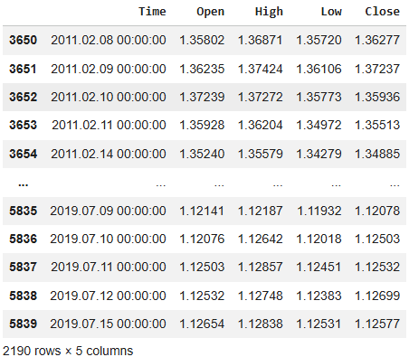

Figure 1: Our historical EURUSD market data.

Let us now create a new target for our prediction. We want to forecast the ratio between the close and open price. If this ratio exceeds 1, then the close price was greater than the open. Otherwise, the open price was greater than the close.

#Generate a target that is a ratio of the data
data["Target"] =  data["Close"] / data["Open"]

Next, we will define our forecast horizon. For today, we will forecast 10 days into the future.

#Set the forecast horizon
HORIZON = 10  

Now we can implement our forecast horizon.

#Shift the target
data["Target"] = data["Target"].shift(-10)

Let us now consider the distribution of our new target. As illustrated in Figure 2 below, our target is centered around 1, with many observations being very close to 1. Additionally, the tail of this distribution is rather tight, except for a few outliers. This suggests that the market may not frequently trend. Otherwise, if the market did trend more frequently, we would've expected a wider distribution that is not centered around 1.

plt.hist(data['Target'],bins=50)
plt.title("Distribution Of The Target")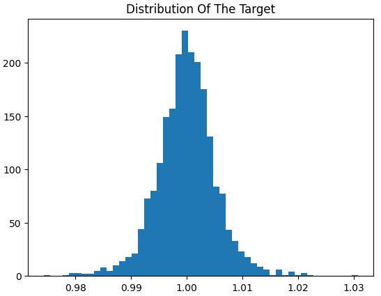

Figure 2: Distribution of the ratio between the open and close price.

Let us partition our data into train and test samples.

#Train test split
train , test = data.iloc[0:data.shape[0]//2,:] , data.iloc[data.shape[0]//2:,:]

Import the statistical learning library we need, along with the model we will use. We will evaluate 6 different models and select the one that performs best on the test set.

#Import statistical models
from sklearn.linear_model import LinearRegression,Ridge,Lasso
from sklearn.ensemble import RandomForestRegressor,GradientBoostingRegressor
from sklearn.svm import LinearSVR
from sklearn.metrics import root_mean_squared_error as RMSE

To evaluate how well our models are performing, we will set a benchmark for our models to surpass. The data is centered around the mean; therefore, we will start by evaluating the error of a naive forecast that always predicts the mean. The standard deviation of the target is the square root of the average dispersion from the mean. This effectively reveals to us the RMSE obtained by forecasting the mean. There is a close relationship between RMSE, standard deviation, and variance.

#Set performance benchmarks
train_benchmark = train['Target'].std()
test_benchmark = test['Target'].std()

Let us initialize the models and collect them.

#Evaluate the models
models = [LinearRegression(),Ridge(),Lasso(),RandomForestRegressor(),GradientBoostingRegressor(),LinearSVR()]

We will need to keep track of our train and test error rates.

train_error = []
test_error = []

Fit each model on the training set, then store both the train and test performance.

for model in models:
  #Fit the model on the training set
  model.fit(train.loc[:,['Open','High','Low','Close']],train['Target'])
  #Evaluate the model
  train_error.append(RMSE(train['Target'],model.predict(train.loc[:,['Open','High','Low','Close']])))
  test_error.append(RMSE(test['Target'],model.predict(test.loc[:,['Open','High','Low','Close']])))

We will evaluate our model's performance on the training sample. Our benchmark is highlighted by a red horizontal line on the graph. On the training set we selected, only one model outperformed the naive forecast. However, this is not enough information to reach a decision. We must also consider how the model performs on the test set.

plt.plot(train_error)
plt.grid()
plt.title('Training Performance')
plt.ylabel('Train RMSE')
plt.axhline(train_benchmark,color='red')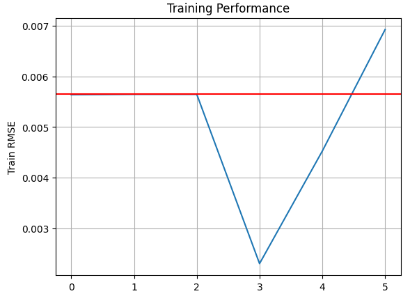

Figure 3: Our model performance on the train set suggests that the Random Forest Regressor is performing well.

On the test set, we obtain the opposite results. The model that had the lowest training error now has the highest test error. This may be an indication of overfitting. Therefore, we will select the linear regressor for our trading strategy.

plt.plot(test_error)
plt.grid()
plt.title('Test Performance')
plt.ylabel('Test RMSE')
plt.axhline(test_benchmark,color='red')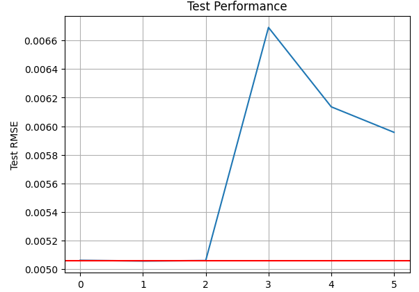

Figure 4: Our performance levels on the test set reveal that our flexible models may have overfit the training data.

Let us now prepare to export our model to ONNX format. ONNX stands for Open Neural Network Exchange. The ONNX specification allows us to build and distribute machine learning models across systems and programming languages without dependencies on the framework used for training.

import onnx
from skl2onnx.common.data_types import FloatTensorType
from skl2onnx import convert_sklearn

Specify the input size expected by the model.

initial_types = [('float_input',FloatTensorType([1,4]))]

And also detail the outputs returned by the model.

final_types = [('float_output',FloatTensorType([1,1]))]

Fit the model on all the historical data we have.

model = LinearRegression()
model.fit(data.loc[:,['Open','High','Low','Close']],data.loc[:,'Target'])

Convert the model to its ONNX prototype and save the model as an ONNX file.

onnx_proto = convert_sklearn(model,initial_types=initial_types,final_types=final_types,target_opset=12)
onnx.save(onnx_proto,'EURUSD_Linear_Regressor.onnx')

Getting Started in MQL5

We will load the ONNX file we saved.

//+------------------------------------------------------------------+
//|                                        EURUSD Mean Reversion.mq5 |
//|                                  Copyright 2026, MetaQuotes Ltd. |
//|                                             https://www.mql5.com |
//+------------------------------------------------------------------+
#property copyright "Copyright 2026, MetaQuotes Ltd."
#property link      "https://www.mql5.com"
#property version   "1.00"

//+------------------------------------------------------------------+
//| System resources                                                 |
//+------------------------------------------------------------------+
#resource "\\Files\\Mean Reverting Strategy\\EURUSD Linear Regressor.onnx" as const uchar onnx_proto[];

Then we will prepare the trade class. The trade class is necessary for efficiently managing our trades. 

//+------------------------------------------------------------------+
//| Library                                                          |
//+------------------------------------------------------------------+
#include <Trade\Trade.mqh>
CTrade Trade;

Our trading strategy has 6 inputs the user can adjust. These inputs have been grouped by functionality. 

//+------------------------------------------------------------------+
//| System inputs                                                    |
//+------------------------------------------------------------------+
input group "Technical Indicators"
input(name="Moving Average Period") int MA_PERIOD = 12;
input(name="ATR Period") int ATR_PERIOD = 14;

input group "Time Frames"
input(name="Higher Time Frame") ENUM_TIMEFRAMES HIGHER_TIME_FRAME = PERIOD_W1;
input(name="Lower Time Frame") ENUM_TIMEFRAMES LOWER_TIME_FRAME = PERIOD_D1;

input group"Risk Management"
input(name="ATR Multiple") double ATR_MULTIPLE = 2;
input(name="Lot Sise") double RISK = 0.01;

We shall define important global variables our application will use in different functions. 

//+------------------------------------------------------------------+
//| Global variables                                                 |
//+------------------------------------------------------------------+
const int magic_number = 2631;
int high_ma,low_ma,daily_high_ma,daily_low_ma,daily_open_ma,daily_close_ma,atr;
double high_ma_reading[],low_ma_reading[],daily_high_ma_reading[],daily_low_ma_reading[],daily_open_ma_reading[],daily_close_ma_reading[],atr_reading[];
double bid,ask,stop_width;
datetime current_timestamp;
vector daily_high,daily_low,daily_open,daily_close;
vectorf model_inputs,model_outputs;
long    model;

On initialization, the Expert Advisor sets a magic number to identify its trades and distinguish them from trades placed manually or by other EAs. After that, it loads the required technical indicators

//+------------------------------------------------------------------+
//| Expert initialization function                                   |
//+------------------------------------------------------------------+
int OnInit()
  {
//--- Set magic number for the application
   Trade.SetExpertMagicNumber(magic_number);

//--- Initialize indicators and test the validty of handlers
   if(!LoadIndicators())
     {
      //--- An error has occured
      Comment("Failed to load indicators correctly: ",GetLastError());
      return(INIT_FAILED);
     }

//--- All is fine
   return(INIT_SUCCEEDED);
  }

If our application is not in use, we will free up all the resources that were previously allocated.

//+------------------------------------------------------------------+
//| Expert deinitialization function                                 |
//+------------------------------------------------------------------+
void OnDeinit(const int reason)
  {
//--- Free up resources
   IndicatorRelease(high_ma);
   IndicatorRelease(low_ma);
   IndicatorRelease(daily_high_ma);
   IndicatorRelease(daily_low_ma);
   IndicatorRelease(daily_open_ma);
   IndicatorRelease(daily_close_ma);
   IndicatorRelease(atr);
   OnnxRelease(model);
  }

When new quotes are received from our broker, we will check if a new daily candle has formed. If this is the case, we will call utility functions that we built to update our technical indicators, manage open positions, or look for entry signals if no position is open.

//+------------------------------------------------------------------+
//| Expert tick function                                             |
//+------------------------------------------------------------------+
void OnTick()
  {
//--- Keep track of time
   current_timestamp = iTime(Symbol(),LOWER_TIME_FRAME,1);
   static datetime time_stamp;

//--- Check if a new candle has formed
   if(time_stamp != current_timestamp)
     {
      //--- Update time stamp
      time_stamp = current_timestamp;

      //--- Copy updated prices and indicator buffers
      if(UpdatePrices())
        {
         //--- Check if we have open positions
         if(TradeExists())
           {
            //--- Manage the open position
            ManagePosition();
           }

         //--- We have no open trades
         else
           {
            //--- Check for entry signal
            CheckTradingSignal();
           }
        }
     }
  }
//+------------------------------------------------------------------+

We manage positions using a trailing stop-loss. The function selects a position by symbol and magic number, then calculates updated SL/TP values based on the position type. It modifies the position only if the stop levels change.

//+------------------------------------------------------------------+
//| Check if we can update our stop levels                           |
//+------------------------------------------------------------------+
void ManagePosition(void)
  {
//--- Select the position
   if(PositionSelect(Symbol()))
     {
      //--- Check the magic number of the position
      if(PositionGetInteger(POSITION_MAGIC) == magic_number)
        {
         //--- Store current SL & TP
         double current_sl,current_tp,new_sl,new_tp;
         current_sl = PositionGetDouble(POSITION_SL);
         current_tp = PositionGetDouble(POSITION_TP);

         //--- Check the position type
         if(PositionGetInteger(POSITION_TYPE) == POSITION_TYPE_BUY)
           {
            new_sl = (bid-stop_width)>current_sl?bid-stop_width:current_sl;
            new_tp = (bids+top_width)>current_tp?bid+stop_width:current_tp;
           }

         //--- Our position is a sell order
         else
           {
            new_sl = (bid+stop_width)<current_sl?ask+stop_width:current_sl;
            new_tp = (bid-stop_width)<current_tp?ask-stop_width:current_tp;
           }

         //--- Check if the position needs modification
         if(new_sl != current_sl)
           {
            Trade.PositionModify(Symbol(),new_sl,new_tp);
           }
        }
     }
  }

Our trading signal is registered first when the price breaks past the weekly moving average. We will then seek additional confirmation from our statistical model and a pair of moving averages we applied to the daily time frame. These moving averages were applied to the daily open and close prices, respectively. If the open moving average is beneath the close, then price levels are tending to open low and close high; this confirms our bullish entry signal. Otherwise, the opposite case confirms our bearish entry signal.

//+------------------------------------------------------------------+
//| Check if our trading signal has formed                           |
//+------------------------------------------------------------------+
void CheckTradingSignal(void)
  {
//--- Long entry conditions
   if((daily_close[0] < low_ma_reading[0]) && (daily_open_ma_reading[0] < daily_close_ma_reading[0]) && (model_outputs[0] > 1))
     {
      //--- Validate the trade was executed
      if(!Trade.Buy(RISK,Symbol(),ask,bid - stop_width,bid + stop_width,""))
        {
         //--- Something went wrong
         Print("Failed to execute buy trade: ",Trade.ResultRetcode()," ",Trade.ResultRetcodeDescription());
        }
     }


//--- Short entry conditions
   else
      if((daily_close[0] > high_ma_reading[0]) && (daily_open_ma_reading[0] > daily_close_ma_reading[0]) && (model_outputs[0] < 1))
        {
         //--- Check if the trade was executed
         if(!Trade.Sell(RISK,Symbol(),bid,ask + stop_width,ask - stop_width,""))
           {
            //--- Something went wrong
            Print("Failed to execute sell trade: ",Trade.ResultRetcode()," ",Trade.ResultRetcodeDescription());
           }
        }
  }

Next, we implement a function to load the indicators and set up the ONNX model. It initializes indicator handles, creates the ONNX model from the embedded buffer, sets input/output shapes, and initializes I/O vectors. It returns false if any handle is invalid; otherwise, it returns true if no errors occurred.

//+------------------------------------------------------------------+
//| Setup Our Technical Indicators                                   |
//+------------------------------------------------------------------+
bool LoadIndicators(void)
  {
//--- Load the required indicators
   high_ma = iMA(Symbol(),HIGHER_TIME_FRAME,MA_PERIOD,0,MODE_EMA,PRICE_HIGH);
   low_ma = iMA(Symbol(),HIGHER_TIME_FRAME,MA_PERIOD,0,MODE_EMA,PRICE_LOW);
   daily_high_ma = iMA(Symbol(),LOWER_TIME_FRAME,MA_PERIOD,0,MODE_EMA,PRICE_HIGH);
   daily_low_ma = iMA(Symbol(),LOWER_TIME_FRAME,MA_PERIOD,0,MODE_EMA,PRICE_LOW);
   daily_close_ma = iMA(Symbol(),LOWER_TIME_FRAME,MA_PERIOD,0,MODE_EMA,PRICE_CLOSE);
   daily_open_ma = iMA(Symbol(),LOWER_TIME_FRAME,MA_PERIOD,0,MODE_EMA,PRICE_OPEN);
   atr = iATR(Symbol(),LOWER_TIME_FRAME,ATR_PERIOD);

//--- Setup the ONNX model
   model = OnnxCreateFromBuffer(onnx_proto,ONNX_DATA_TYPE_FLOAT);

//--- Define the model parameter shape
   ulong input_shape[] = {1,4};
   ulong output_shape[] = {1,1};

   OnnxSetInputShape(model,0,input_shape);
   OnnxSetOutputShape(model,0,output_shape);

//--- Initialize model inputs and outputs
   model_inputs = vectorf::Zeros(4);
   model_outputs = vectorf::Zeros(1);

//--- This function will return false if any of the indicators failed to load
   return((model != INVALID_HANDLE)||(high_ma != INVALID_HANDLE)||(low_ma != INVALID_HANDLE)||(atr != INVALID_HANDLE)||(daily_close_ma != INVALID_HANDLE)||(daily_open_ma != INVALID_HANDLE)||(daily_high_ma != INVALID_HANDLE)||(daily_low_ma != INVALID_HANDLE));
  }
//+------------------------------------------------------------------+

Once that is complete, we define a function that checks whether we have any open trades. The function first filters all open positions based on the trading symbol. It then filters the remaining positions using the magic number that was set during initialization.

This magic number is a unique identifier for all trades placed by our Expert Advisor. It allows us to distinguish between trades placed by this specific Expert Advisor and those placed manually by the user or by other Expert Advisors that the user may be running.

The function returns a Boolean value that indicates whether a matching position has been identified. If the function returns false, no matching position was found, meaning that there are no open trades. Conversely, if the function returns true, an open position has been identified, and the trade must be managed accordingly.

//+------------------------------------------------------------------+
//| Check if we have already placed a trade                          |
//+------------------------------------------------------------------+
bool TradeExists(void)
  {
//--- Get trades for the current symbol
   if(PositionSelect(Symbol()))
     {
      //--- Check the magic number
      if(PositionGetInteger(POSITION_MAGIC) == magic_number)
        {
         //--- We have a position that is still open
         return(true);
        }
     }
//--- We have no open positions
   return(false);
  }
//+------------------------------------------------------------------+

Next, we define a method that updates prices and indicator values by copying the latest readings from indicator handles into the corresponding buffers.

The method attempts to call the CopyBuffer() function and, if an error occurs, provides feedback by printing an error message to the console. The method also returns a Boolean flag that is false if an error has occurred and true otherwise. Trading activity is suspended for a day in the event of an error.

After successfully copying the indicator readings into their respective buffers, we set each indicator buffer as a series. We also keep track of the bid and ask prices as they continue to evolve. Additionally, we maintain vectors that store the daily high, low, open, and close prices. These vectors are updated each day.

Finally, we obtain a prediction from our ONNX model. If this step is completed successfully, we perform the final calculation of the stop-loss level that will be used for our symmetric stop-loss and take-profit system by using the current ATR reading.

//+------------------------------------------------------------------+
//| Update our prices and indicator buffers                          |
//+------------------------------------------------------------------+
bool UpdatePrices(void)
  {
//---- Copy udated indicator reading to buffer
//--- High MA indicator
   if(CopyBuffer(high_ma,0,1,12,high_ma_reading) <= 0)
     {
      //--- Failed to read in the moving average high indicator
      Print("Failed to read the weekly moving average high indicator buffer: ",GetLastError());
      return(false);
     }
//--- Low MA indicator
   if(CopyBuffer(low_ma,0,1,12,low_ma_reading) <= 0)
     {
      //--- Failed to read in the moving average low indicator
      Print("Failed to read the weekly moving average low indicator buffer: ",GetLastError());
      return(false);
     }
//--- Daily High MA indicator
   if(CopyBuffer(daily_high_ma,0,1,1,daily_high_ma_reading) <= 0)
     {
      //--- Failed to read in the daily moving average high indicator
      Print("Failed to read the daily moving average high indicator buffer: ",GetLastError());
      return(false);
     }
//--- Daily Low MA indicator
   if(CopyBuffer(daily_low_ma,0,1,1,daily_low_ma_reading) <= 0)
     {
      //--- Failed to read in the daily moving average low indicator
      Print("Failed to read the daily moving average low indicator buffer: ",GetLastError());
      return(false);
     }
//--- Daily Open MA indicator
   if(CopyBuffer(daily_open_ma,0,1,1,daily_open_ma_reading) <= 0)
     {
      //--- Failed to read in the daily moving average open indicator
      Print("Failed to read the daily moving average open indicator buffer: ",GetLastError());
      return(false);
     }
//--- Daily Close MA indicator
   if(CopyBuffer(daily_close_ma,0,1,1,daily_close_ma_reading) <= 0)
     {
      //--- Failed to read in the daily moving average close indicator
      Print("Failed to read the daily moving average close indicator buffer: ",GetLastError());
      return(false);
     }
//--- ATR indicator
   if(CopyBuffer(atr,0,1,1,atr_reading) <= 0)
     {
      //--- Failed to read in the ATR indicator
      Print("Failed to read the daily ATR indicator buffer: ",GetLastError());
      return(false);
     }

//--- Set the moving average buffer as series
   if(!ArraySetAsSeries(high_ma_reading,true))
     {
      //--- We failed to set the high moving average buffer as series
      Print("An error occured when organizing the high moving average buffer: ",GetLastError());
      return(false);
     }

   if(!ArraySetAsSeries(low_ma_reading,true))
     {
      //--- We failed to set the low moving average buffer as series
      Print("An error occured when organizing the low moving average buffer: ",GetLastError());
      return(false);
     }

//--- Keep track of current bid & ask prices
   if(!SymbolInfoDouble(Symbol(),SYMBOL_BID,bid))
      {
         //--- An error occured reading the bid price
         Print("An error occured reading the bid price: ",GetLastError());
         return(false);
      }
   if(!SymbolInfoDouble(Symbol(),SYMBOL_ASK,ask))
       {
         //--- An error occured reading the ask price
         Print("An error occured reading the ask price: ",GetLastError());
         return(false);
      }

//--- Copy historical price levels to vector
//--- High
   if(!daily_high.CopyRates(Symbol(),LOWER_TIME_FRAME,COPY_RATES_HIGH,1,30))
     {
      //--- Failed to copy the historical daily high price
      Print("Failed to copy the historical daily high price to vector: ",GetLastError());
      return(false);
     }
//--- Low
   if(!daily_low.CopyRates(Symbol(),LOWER_TIME_FRAME,COPY_RATES_LOW,1,30))
     {
      //--- Failed to copy the historical daily low price
      Print("Failed to copy the historical daily low price to vector: ",GetLastError());
      return(false);
     }
//--- Open
   if(!daily_open.CopyRates(Symbol(),LOWER_TIME_FRAME,COPY_RATES_OPEN,1,30))
     {
      //--- Failed to copy the historical daily open price
      Print("Failed to copy the historical daily open price to vector: ",GetLastError());
      return(false);
     }
//--- Close
   if(!daily_close.CopyRates(Symbol(),LOWER_TIME_FRAME,COPY_RATES_CLOSE,1,30))
     {
      //--- Failed to copy the historical daily close price
      Print("Failed to copy the historical daily close price to vector: ",GetLastError());
      return(false);
     }

//--- Prepare ONNX model inputs
   model_inputs[0] = (float)iOpen("EURUSD",PERIOD_D1,0);
   model_inputs[1] = (float)iHigh("EURUSD",PERIOD_D1,0);
   model_inputs[2] = (float)iLow("EURUSD",PERIOD_D1,0);
   model_inputs[3] = (float)iClose("EURUSD",PERIOD_D1,0);

//--- Obtain ONNX model forecast
   if(!(OnnxRun(model,ONNX_DATA_TYPE_FLOAT,model_inputs,model_outputs)))
     {
      Comment("Failed to obtain a forecast from our model: ",GetLastError());
     }

   else
     {
      Comment("Forecast: ",model_outputs);
     }

//--- Calculate the new stop levels
   stop_width = NormalizeDouble(((atr_reading[0] * ATR_MULTIPLE) + (SymbolInfoInteger(Symbol(),SYMBOL_TRADE_STOPS_LEVEL) * _Point)),_Digits);

//--- Everything went fine
   return(true);
  }
//+------------------------------------------------------------------+

Backtesting Our Expert Advisor

We are now ready to begin backtesting our trading strategy. In the figure below, we have included a screenshot of the inputs that our Expert Advisor accepts from the end user. You may adjust these inputs as needed to suit your trading preferences or testing requirements.

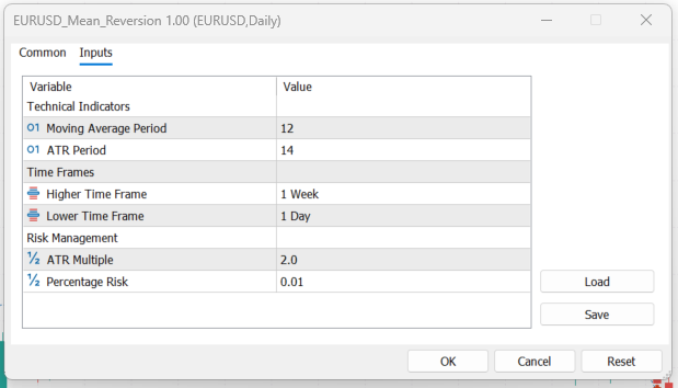
Figure 5: Selecting the inputs for our trading strategy.

Next, we will select the backtesting period, which ranges from 2020 to 2026, to evaluate our application using historical market data. Be sure to select the correct time frame that corresponds with the inputs you provided for the application, as this will ensure that the strategy is tested under the intended market conditions.

Figure 6: The backtest will run from 2020 until 2026. This is the out-of-sample period we reserved for testing.

For our backtest to be reliable, it must be as realistic as possible. Therefore, we will model market performance using real ticks. This ensures that we are using the most accurate historical data available. Additionally, we will set the execution delay to Random Delay. This emulates the market latency that is typically experienced during real trading, resulting in a more realistic evaluation of the strategy's performance.

Figure 7: The test conditions have been selected to emulate the experience of real trading.

When we observe the equity curve produced by our trading strategy, we can see that the strategy has a positive effect on the account equity over time. The reader should recall that our statistical model of the market was trained using data from 2011 to 2019. Consequently, the results presented here represent the out-of-sample performance of our strategy over a six-year period.

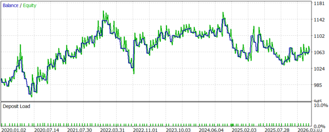
Figure 8: The equity curve produced by our trading strategy.

Lastly, we have produced a detailed statistical analysis of the performance of our trading strategy over the six-year backtest. By examining the statistical results, we observe that the average profitable trade was almost 50% larger than the average losing trade. Additionally, the largest profit realized was substantially greater—almost twice as large as the largest loss incurred by the strategy during the backtest. The strategy also produced a profit factor of 1.1, indicating that it is expected to appreciate the account balance over time, provided that similar market conditions persist.

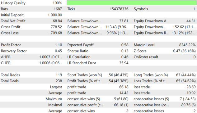
Figure 9: A detailed analysis of our trading performance.

Conclusion

This article has demonstrated how to build a mean-reversion trading strategy for the MetaTrader 5 platform using MQL5 and standard Python libraries. After reading this article, the reader will have a template for identifying mean-reverting markets based on the distribution of returns, as demonstrated earlier in the discussion.

Additionally, the reader is equipped with an integrated framework for building ensemble trading strategies that combine the strengths of both MQL5 and Python. In our next discussion, we will build upon the baseline performance established in this article and explore techniques for outperforming the benchmark that we have set.

File Name	Description
EURUSD_Mean_Reversion.ipynb	The Jupyter notebook we built to analyze the historical EURUSD market data we fetched and to build our ONNX model. The notebook is contained inside the Python Code.zip attached file.
EURUSD_Linear_Regressor.onnx	The statistical model we built based on historical EURUSD market data. The ONNX file is contained in the MQL5.zip file, under the Files subfolder; all files are attached below.
EURUSD_Mean_Reversion.mq5	Our trading application that employed a combination of technical analysis and statistical modeling. The Expert Advisor is housed in the MQL5.zip file, under the Experts subfolder; all related files are attached below.
EURUSD Mean Reversion Data.mq5	This is the MQL5 script we implemented to fetch historical data and write it out to a CSV file. The script is found in the MQL5.zip file, under the Scripts subfolder; all related files are attached below.