The Hypothesis of Randomness: Searching for Hidden Patterns in Price Series

Introduction

In statistical problems, the input data are often treated as a random sample from a certain distribution; that is, the components of the data vector are considered to be independent and identically distributed random variables. In many problems, this assumption is uncontroversial, since it follows from the nature of the data itself. But sometimes this initial assumption itself needs to be tested and is treated as a statistical hypothesis known as the hypothesis of randomness.

A classic example is quality control of pseudorandom number generators (PRNGs). Software algorithms generate sequences that must be statistically indistinguishable from truly independent and uniformly distributed random variables on the unit interval [0,1]. Therefore, the quality of PRNG output must be monitored, which ultimately amounts to testing the hypothesis of randomness.

Testing this hypothesis on the quotes of financial instruments can provide valuable information to analysts who develop trading systems based on detecting statistically significant deviations from the efficient market hypothesis. This article examines how to test the randomness hypothesis using the chi-square method. This is a versatile and well-studied method that can be used to test various statistical hypotheses; it is based on comparing the observed and expected frequencies of events. Most importantly, it is relatively easy to put into practice.

Problem Statement

So, let us consider a sequence of n random variables (ξ₁, ξ₂, ..., ξₙ) that take values from a finite set (alphabet) E = {1, 2, ..., N}, and suppose we want to test the hypothesis that these variables are independent and uniformly distributed, that is, P{ξi=j} = 1/N, j = 1, ..., N, i = 1, 2, ..., n. This is the null hypothesis for an ideal random number generator.

One suitable method for testing such a hypothesis is the chi-square test. It is based on counting so-called s-chains (s-grams or s-tuples) in a random sequence. An s-chain is defined as any subsequence of a sequence of random variables consisting of s consecutive terms. For example: (ξ1, ..., ξs), (ξ2, ..., ξs+1), …, (ξn-s+1, ..., ξn), for a total of n - s + 1 chains. Instead of considering the frequencies of individual outcomes in a sequence, we consider the frequencies of outcome chains of a fixed length s ≥ 1, where the chains must overlap.

Let i_ = (i1, …, is) be any s-tuple of elements of the set E; then there are N^s such tuples in total. For example, let N = 2 (E = {0, 1}) and s = 2; then we get 4 tuples: {(0, 0), (0, 1), (1, 0), (1, 1)}. The frequencies of the s-chains and (s+1)-chains are calculated using the following formulas:

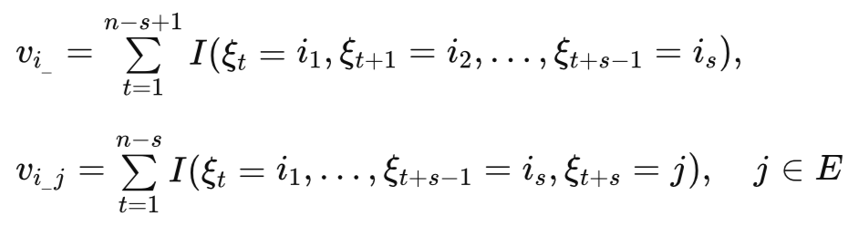
where I(A) is the indicator of event A.

At the same time, in practice, it is sufficient to compute only the frequencies of the (s+1)-chains {vi_j} (there are N^(s+1) of them), since:

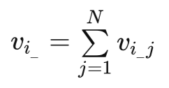
Although the sum of the frequencies of the s-chains calculated in this way may differ from the true value by one, this does not affect the chi-square statistic; however, it does reduce the computational effort by counting only the (s+1)-chains.

To test the null hypothesis of randomness using the chi-square statistic, the empirical frequencies vi_j are compared with the expected frequencies (vi_/N):

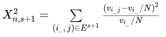
where (i_j) is a specific (s+1)-chain.

Explanation of How the Algorithm Works

To understand whether there is a pattern in the data, we need to compare what we observe in reality with what we would expect to see in the case of perfect chaos. If we take a fair coin as a model of perfect chaos (the set of states consists of 2 points, E = {0, 1}), then:

• the probability of any state occurring:

P(j) = 1/N = 1/2

• the probability of observing any s-tuple i_ = (i1, …, is):

P(i_) = 1/N^s

• the expected frequency of a given event:

Evi_ = n/N^s

• the probability of observing state j after the s-dimensional combination i_ (according to the multiplication rule for independent events):

P(i_, j) = P(i_) * P(j) = 1/N^s * 1/N = 1/N^(s+1)

Let's say we take a specific sequence of s candlesticks — for example, two white candlesticks in a row (1,1) — and look at what happened immediately after them. Suppose this situation occurred in the historical data vi_ = 1,000 times. Of these, 600 times the next candle was white (j=1), and 400 times it was black (j=0), so the empirical frequencies vi_j are vi_j(1,1,1) = 600 and vi_j(1,1,0) = 400.

If the market is completely random and has no memory of the past, then after any pattern — regardless of how often that pattern occurred on its own within the sample — the probability of an up or down move should remain 0.5.

In our example, the pattern vi_(1,1) occurred 1,000 times. Thus, out of 1,000 cases, we expect to see exactly 500 outcomes in each direction. The quantity vi_ * 1/N is the conditional expected frequency.

By summing the normalized squares of the deviations of the observed frequencies from these expected values across all possible combinations (i_j), we obtain a final value — the chi-square statistic. This statistic is, in and of itself, a random variable, since it depends on the specific data sample.

In his work Statistical Inference for Markov Processes (1961), the American mathematician Billingsley proves that, assuming the null hypothesis is true, this statistic has a limiting chi-square distribution with N^s*(N-1) degrees of freedom.

The test defined at a significance level alpha by the critical region {Xn, s+1 > Chi2(1-alpha), N^s*(N-1)} is consistent against alternatives in which the sequence of random variables is a homogeneous ergodic Markov chain of order s.

Recall that a Markov chain is called homogeneous if the transition probabilities in the chain do not depend on time. This concept is, in a sense, analogous to stationarity in the theory of stationary random processes, where it is assumed that the statistical characteristics of the process remain constant over time. Therefore, when dealing with non-stationary processes, this must be taken into account: we should look for periods of quasi-stationarity where we believe the process characteristics do not change significantly, and identify homogeneous segments of the time series — for example, within a single trading session (Asia, Europe, America), etc.

A Markov chain is called ergodic if the limits of the probabilities of the combinations i_ = (i1, …, is) exist and do not depend on the initial distribution of the chain. In this case, for a chain to be ergodic, it is sufficient that all transition probabilities be positive (that is, all transitions are possible in the chain).

Applying this criterion to the analysis of quotes allows us to interpret market dynamics as a Markov process. By analyzing the chi-square statistic, we are essentially testing the hypothesis of whether the candlestick sequence is white noise or is generated by a homogeneous ergodic Markov chain of order s. The ergodicity condition (the presence of all possible transitions in the data) guarantees the consistency of the test, allowing it to reveal hidden patterns — market memory — that are inaccessible to classical methods of correlation analysis.

Implementation of the Algorithm in Python

The basis for implementing the algorithm is the Counter class. This is a specialized dictionary subclass located in the collections module and specifically designed for quickly counting repeated elements. In our case, we will group market patterns and count their occurrences. Specifically:

• keys are the patterns themselves (s-chains / s-tuples of the random sequence),
• values are the number of their repetitions (how many times the pattern appeared in the history)

Here is a clear example of how Counter processes a sequence of candles when s=2 (when we are looking for the influence of the two previous candles on the current one). Let’s consider a short segment of quotes consisting of 6 bars: 1, 1, 0, 1, 1, 1 (where 1 indicates an increase and 0 indicates a decrease).

from collections import Counter 

# Our sequence (6 candles) 
sequence = [1, 1, 0, 1, 1, 1] 
s = 2 

# 1. Collect (s+1)-chains / (s+1)-tuples (triples) using a sliding window: 
# [1, 1, 0], 1, 1, 1 -> (1, 1, 0)
# 1, [1, 0, 1], 1, 1 -> (1, 0, 1) 
# 1, 1, [0, 1, 1], 1 -> (0, 1, 1) 
# 1, 1, 0, [1, 1, 1] -> (1, 1, 1)

 patterns = [(1,1,0), (1,0,1), (0,1,1), (1,1,1)] 

# 2. Create a Counter object: 
v_ij_counts = Counter(patterns)

 print(v_ij_counts)
 # Result: Counter({(1,1,0): 1, (1,0,1): 1, (0,1,1): 1, (1,1,1): 1}) 

As a result, when we feed a real sequence as input, we will get something like this:

{
 (1, 1, 1): 450, # The “three consecutive up moves” pattern occurred 450 times 
(1, 1, 0): 120, # The “two up moves and a reversal” pattern occurred 120 times 
(0, 0, 1): 380, # The “two drops and a rebound” pattern occurred 380 times 
# ... and so on for all combinations
 } 

To perform the calculations, we will need the function `chi2_randomness(sequence, s, alpha=0.05)`, which takes as input a discrete sequence, the Markov chain order `s`, and the significance level `alpha` (the probability of a Type I error).

def chi2_randomness(sequence, s, alpha=0.05):
    """
    Chi-square test for the presence of Markov memory in the discrete sequence
    Args:
        sequence: Discrete sequence 
        s: Markov chain order (memory depth)
        alpha: Significance level
        
    Returns:
        Dict: Statistics, critical value, p-value etc.
    """
    n = len(sequence) # the number of elements in the sequence under study
    if n <= s:
        return {
            "statistic": 0.0, "critical_value": 0.0, "p_value": 1.0,
            "is_rejected": False, "df": 0, "warning": "Sequence too short"
        }
    
    alphabet = sorted(list(set(sequence))) # automatically determines the system alphabet (set E)
    N = len(alphabet) # number of elements in E
    
    # 1. Count only the frequencies of (s+1)-chains (v_ij): N^{s+1} combinations
    v_ij_counts = Counter() # Create a Counter object
    for t in range(n - s):
    # Iterate through the entire history using a window of length s+1. Each combination found is stored as a tuple
        chain_s_plus_1 = tuple(sequence[t : t + s + 1]) # create a key for an (s+1)-chain
        v_ij_counts[chain_s_plus_1] += 1 # If the pattern is encountered for the first time, the Counter object will create a new record
        
    # 2. To obtain the frequency v_i, sum the frequencies v_ij for all j with the given prefix i
    v_i_from_v_ij = Counter() # Create a Counter object
    for chain_s_plus_1, count in v_ij_counts.items():
        prefix_i = chain_s_plus_1[:-1] # Create a new key: take the first s elements
        v_i_from_v_ij[prefix_i] += count # We calculate the frequency v_i

    # 3. Calculate the chi-square statistic 
    chi_square_stat = 0
    
    # Iterate in a loop over all encountered s-chains (i)
    for i_chain, v_i in v_i_from_v_ij.items():       
        expected = v_i / N # Expected value under H0: v_i / N (equal probability)
        # For each i-chain, consider all possible continuations j from the alphabet (set E)
        for j_state in alphabet:
            ij_chain = i_chain + (j_state,)
            v_ij = v_ij_counts.get(ij_chain, 0)             
            chi_square_stat += ((v_ij - expected)**2) / expected
   
    df = (N**s) * (N - 1) # Degrees of freedom: N^s(N - 1)
    critical_value = chi2.ppf(1 - alpha, df) 
    p_value = 1 - chi2.cdf(chi_square_stat, df)
    
    return {
        "statistic": chi_square_stat,
        "critical_value": critical_value,
        "p_value": p_value,
        "is_rejected": chi_square_stat > critical_value, 
        "df": df
    }

Note that in the loop `for j_state in alphabet:`, we iterate through all possible scenarios. For example, if there has never been a 0 in the sequence under study following the combination (1, 1), we are still required to check this case in order to correctly calculate the deviation from randomness. Using the get(..., 0) method, we set the frequency to zero for those combinations (i_j) that did not occur but could theoretically have occurred.

Interpretation of the results obtained:

• Statistic — the final value of the chi-square statistic,
• critical_value — the critical value of the statistic; if our chi-square statistic is greater than this number, the randomness hypothesis is rejected,
• p_value — the computed probability of error; if it is less than the specified alpha value, we conclude that there is memory in the data and, consequently, reject the randomness hypothesis,
• df — calculation of the number of degrees of freedom; this represents the complexity of our model — the larger the value of s, the greater the number of degrees of freedom.

Quantile Transformation of a Series

To apply the test correctly to market quotes, we will need the quantile_transform(data, n_states=2) function, which performs a quantile transformation of a real-valued series. It allows real-valued data to be mapped to a discrete set with guaranteed equal probability of states. Instead of simply dividing the market into rises and falls relative to zero (which often introduces distortions due to trends), this function splits the data into N states based on empirical quantiles. In the binary case (N=2), the median of the series serves as the classification threshold. As a result, each state (0, 1, 2...) will occur in the sample with the same frequency (P(Ej) ≈ 1/N).

def quantile_transform(data, n_states=4)-> np.ndarray:
    """
    Quantile transformation divides real data 
    by N discrete states based on empirical quantiles.
    This neutralizes the trend influence and provides P{E(j)} = 1/N
    
    Args:
        data: One-dimensional array of real numbers (increments, returns)
        n_states: Number of discrete states (alphabet size)
        
    Returns:
        np.ndarray: Sequence of integers (state indices) from 0 to N-1
    
    """
    # Calculate the thresholds for N states
    # For n_states=4, the thresholds will be at 25%, 50%, and 75%
    quantiles = np.linspace(0, 100, n_states + 1)[1:-1]
    thresholds = np.percentile(data, quantiles)
    
    # Convert the data into a sequence of states 0, 1, ..., N-1
    return np.digitize(data, thresholds) 

The reader may have a reasonable question: why artificially eliminate asymmetry if it is an advantage for us? After all, if we see 60% white candlesticks in the historical data, why not simply keep betting on a rise? Of course, the asymmetry of the process is also a form of market knowledge, but it is primitive knowledge. You do not need complex tests or Markov chains to use it — a buy-and-hold strategy is enough. We, however, want to focus on identifying hidden Markov dependence — that is, how the past influences the future, regardless of the overall direction of price movement.

As an example, let's look at an experiment that can be found in the `randomness.py` module. There, we take a real-valued series generated by a normal distribution with mean μ = 0.5 (a clear upward trend) and standard deviation σ = 1.0. If we simply split the series based on whether the values are greater than or less than zero, we will end up with a clear bias toward ones (growth). Our chi-square test will detect an anomaly and yield a low p-value, indicating non-randomness.

But this will be a false alarm: the data contains no memory; there is only a drift in the mean. Using the `quantile_transform` function, we will find the median of this series (in our example, it will be around 0.5) and use it as our reference point. Values above 0.5 are mapped to 1, and values below 0.5 to 0. As a result, we will obtain a perfect balance of states (for example, 500 zeros and 500 ones in a sample of 1,000 data points). Now, if the chi-square test yields a low p-value, this will indicate something far more significant: the sequence of events has an underlying structure that cannot be explained by a simple mean shift. Thus, quantile transformation makes it possible to separate the market’s trend component from its memory.

It is worth noting that when testing PRNGs (pseudorandom number generators), quantile transformation is not required, since an ideal generator must, by definition, produce a uniform distribution. But for market quotes, this is the only way to filter the trend out of the series and focus exclusively on the transition dynamics.

This module also examines a Markov chain model that can be described by a doubly stochastic transition probability matrix, where the probability of a state change (from 0 to 1 or from 1 to 0) is high — 0.9 — while the probability of remaining in the current state is only 0.1 (Fig. 1).

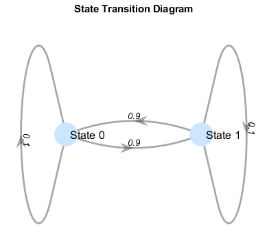
Fig. 1. Graph of a Markov chain with two states and transition probabilities

The mathematical property of such a system is that, in the long run (in the limit), the frequency of occurrence of each state will tend toward 0.5. In other words, when we look at the final statistics for the sequence, we'll see a perfect balance: 50% zeros and 50% ones. Nevertheless, this sequence is anything but random. Knowing that the current state is 0, we can predict with 90% probability that the next state will be 1.

This example shows that we need to distinguish between the frequency distribution of states (how many zeros and ones there are) and the transition structure (the order in which they follow one another). That is why there may not be a trend in market quotes, but patterns may hypothetically exist within a series — in other words, the series may have "memory."

Does EURUSD Have a "Memory"?

For this experiment, let's use the daily quotes for the EURUSD currency pair. The sample size was approximately 1,000 trading days (about 4 years of up-to-date market history, with the last date being 2026-04-03). The data were first preprocessed to remove the trend using a quantile transformation, which brought them into a balanced form: 500 instances of a decline (0) and 501 instances of an increase (1).

We tested the randomness hypothesis for three levels of memory depth (s = 1, 2, 3).

The results turned out to be quite unexpected:

Chain order s	Chi-square statistic	P-value	Memory detected
s=1	0.04	0.98	no
s=2	3.98	0.41	no
s=3	18.18	0.02	yes

It turns out that, on the daily timeframe, EURUSD behaves like a completely random process when examining a memory depth of 1 or 2 steps. However, as soon as we increased the analysis depth to 3 days, the chi-square statistic led us to reject the null hypothesis of randomness (p-value = 0.019, which is below the critical threshold of α = 0.05). This means that the structure of the previous three days has a statistically significant effect on the fourth day. The probability that such a dependence arose by chance is less than 2%.

By running the EURUSD_D.py script, you can analyze exactly which candlestick combinations create this non-randomness by examining the pattern table (this is handled by the analyze_patterns(sequence, s_order) function). This table lists the patterns with the greatest deviation from the theoretical expected frequencies under the null hypothesis (the top 10 combinations out of 2^4 = 16).

The top-ranked pattern is (1, 1, 0, 0). In theory, it should have occurred 62 times on average, but in reality it appeared 84 times (a deviation of +34.6%). This indicates a steady market tendency toward a certain cyclical inertia after two days of gains and one day of losses.

The pattern (0, 1, 0, 0) comes in second place. It occurred only 45 times instead of the expected 62 (a deviation of -27.8%). For some reason, the market avoids this combination.

To definitively verify that the algorithm works correctly, we will use a permutation test. Using the permutation function from NumPy, we completely shuffled the sequence of EURUSD price increments, breaking the chronological relationship between days while preserving the original balance of zeros and ones.

• Actual sequence: p-value = 0.01989 (the sequence is not random)
• Shuffled sequence: p-value = 0.42883 (the sequence is random)

The fact that, after randomizing the series, the p-value immediately returned to the region consistent with randomness (≈0.43 > 0.05) confirms that the algorithm is working correctly. The anomaly found in the real data is due solely to the market’s temporal memory, which disappears when the order of the candlesticks is disrupted.

Thus, the most recent 1,000 daily EURUSD price increments exhibit behavior that is not white noise. This segment of the time series exhibits a hidden third-order structure, and the identified patterns (such as 1, 1, 0 → 0) represent an example of market inefficiency.

Nevertheless, despite the statistical significance of the result in the current segment of historical data, the detected inefficiency disappears when the time window is shifted 1,000 bars back into the past. Readers can easily verify this for themselves.

mt5.copy_rates_from_pos(symbol, timeframe, 0, count) →  mt5.copy_rates_from_pos(symbol, timeframe, 1000, count) 

This fact once again confirms that prices of financial instruments are non-stationary processes. Their probabilistic characteristics are not fixed once and for all; instead, they drift and transform as market regimes change and market participants' behavior shifts.

To replicate the experiments, you will need a Python interpreter (version 3.10+ is recommended) and a standard set of libraries for data analysis.

1. Installing Python. Download the latest version of Python from the official website at https://www.python.org/downloads/windows

2. Installing the required packages. Open the Command Prompt (CMD) and install the libraries with a single command:

pip install numpy pandas scipy MetaTrader5 

3. Project structure. For convenience, I split the code into two files. Place them in a single folder (for example, Scripts/RandomnessTest):

• randomness.py is a library file (module) containing the mathematical functions needed to compute the chi-square test, as well as examples from the article.
• EURUSD_D.py — the main script for testing the randomness hypothesis. It connects to MetaTrader 5, retrieves quotes, and calls functions from the first file for analysis.

4. How to run the analysis:

• open the MetaTrader 5 terminal and run the script or module simply by double-clicking the file in File Explorer,
• all calculations (the chi-square statistic, p-value, number of patterns found, etc.) will be displayed in the “Experts” tab of the terminal.

Conclusion

Using the chi-square test to test the randomness hypothesis allows a trader to move from an intuitive search for patterns to a rigorously grounded mathematical verification of the hypothesis that memory is present in price series.

The algorithm developed is capable of finding memory in the data, provided that such memory actually exists. At the same time, thanks to the quantile transformation, the method successfully ignores data asymmetry and does not generate false signals where no statistical dependence is present.

Undoubtedly, the non-stationarity of financial markets imposes certain limitations on the application of any statistical test. However, this does not diminish the value of the method; rather, it underscores the need to use it adaptively and cautiously — for example, by regularly reevaluating it using sliding windows.

We hope that the proposed approach will take its rightful place in the arsenal of algorithmic traders, helping them distinguish true market inefficiencies from random noise.

Programs used in the article:

#	Name	Type	Description
1	randomness.py	Script	A module containing the functions needed to test the randomness hypothesis
2	EURUSD_D.py	Script	Analysis of the randomness hypothesis using daily EURUSD quotes as an example