Neural Networks in Trading: A Spike-Semantic Approach to Spatiotemporal Identification (Conclusion)

Introduction

Just because the market is quiet does not mean it is calm. Beneath its smooth surface, life is constantly bubbling: bursts of orders, tremors in liquidity, and shifts in trading volume. All of this consists of brief, almost imperceptible impulses that give rise to price movements. Every tick is a signal in the living fabric of the market. And it is precisely in those moments, when most people still see only silence, that the real process of trend formation begins.

Traditional methods of analysis are too slow to capture this moment. They see only a fait accompli — a candlestick, an extremum, a pattern. But what matters to a trader is something else: sensing a change before it becomes obvious. And this is where the new generation of models comes in — architectures capable of recognizing events.

One such architecture is S3CE-Net — Spike-guided Spatiotemporal Semantic Coupling and Expansion Network. It was originally designed to process data streams from event cameras, where each pixel captures not a static image but an instantaneous change in light — a sort of spike or pulse. Essentially, these are the same events as those in the market: irregular, asynchronous, brief, yet significant.

We wondered: after all, the financial market is an event-driven system too. Time does not flow uniformly here. Everything is determined by bursts of activity — moments when a major player suddenly appears in the order flow, liquidity tightens, and the price accelerates. If we teach the model to perceive these impulses as a structure, it will be able to anticipate and react.

In previous articles, we have already explored the theoretical foundation of the S3CE-Net framework. We considered the concept of the event-driven approach, explained why the market can be viewed as a stream of impulses, and laid the groundwork for implementing the proposed approaches in the MQL5 environment.

The next stage was an engineering step forward: we implemented the SSAM (Spike-guided Spatial-Temporal Attention Mechanism) module and adapted it to the computational characteristics of the trading terminal.

Now it is time for the final stage. Here, we bring everything together — from concept to practice, from event theory to evaluating the results. We will examine how S3CE-Net behaves on real historical data, how resilient it is to market noise, and whether its attention can distinguish true signals from random fluctuations.

The S3CE-Net architecture is based on two complementary ideas. The first is SSAM, an attention mechanism that learns to focus on important events and suppress insignificant ones. It is like an experienced trader who can discern market sentiment behind the flow of candlestick patterns — where momentum is full of energy and where it is merely a fading wave. The second is STFS (Spatiotemporal Feature Sampling Strategy). It broadens the model’s perception, allowing it to see a smooth sequence of interconnected events.

To draw an analogy, SSAM is a trader’s attention, and STFS is the trader’s memory. Together, they form a model that can notice and remember what happened before. This is the true essence of analysis: not getting stuck in the moment, while also not losing touch with the context.

When we transfer these ideas into the MQL5 environment, the challenge becomes not only technical but also philosophical. A video camera records changes in brightness, while the market captures changes in the state of price and volume. Every tick, every spike in volatility, every change in the order book — all of these can become a spike if the significance criterion is defined correctly.

This approach makes you look at the market differently. We see a system of impulses from which a macro-movement is formed. S3CE-Net seems to translate market speech into the language of events, where each change is a letter and the entire series is a sentence. The model learns to read this language the way an experienced analyst reads a tape chart: not with their eyes, but by intuition. S3CE-Net does not wait for a pattern to be confirmed — it reacts to precursors. This is especially important in highly volatile markets, where traditional indicators lag behind.

To a trader who is used to relying on candlestick patterns or indicators, this idea may seem unfamiliar. But if you look more closely, it is a logical continuation of the evolution of analysis. First, we assessed levels and zones; then we moved on to probabilistic models; now it is time for event-driven models. It is a natural progression — from observation to understanding, from data to meaning.

That is precisely why the work on implementing S3CE-Net using MQL5 is not limited to purely technical goals. We aim to show how architectural principles developed for a completely different field can breathe new life into market analysis. After all, both trading and event-driven analytics are about searching for structure in chaos — the ability to extract meaning from the flow.

The market, like any living system, breathes unevenly, and whoever can hear this rhythm gains an advantage. S3CE-Net is an attempt to give machines this sense of hearing — to enable an algorithm to sense where movement begins and where it ends. This is not magic — it is the result of a careful analysis of the structure of events.

The author’s visualization of the S3CE-Net framework is shown below.

Today we are approaching the logical conclusion. The architecture, implementation, and adaptation are now behind us. Ahead lie testing, evaluation, and, perhaps, a rethinking of our usual approach to forecasting. We will see how well the model we have built handles real-world market flows, how accurately it distinguishes genuine signals, and how its spike-guided attention affects the quality of its forecasts.

STFS Module

Today, we have one final step left to take in implementing the approaches proposed by the authors of the S3CE-Net framework: to build the STFS (Spatio-Temporal Feature Sampling Strategy) module. This is the final component of the entire architecture, capable of teaching the model to view the market holistically — to perceive the broader context rather than becoming fixated on local patterns.

Like any experienced trader, STFS learns to distinguish what matters from what is secondary. Its task is to make the model analyze not only specific segments of market data, but also the relationships between them, combining the perception of time and space. After all, the market is not just a line on a chart. It is a multidimensional system in which every candle, every volume reading, and every impulse are linked by invisible threads. It is precisely these connections that the algorithm must learn to recognize.

The authors of S3CE-Net proposed a very elegant mechanism for this. During training, the module divides the feature map into subsamples along the time and spatial dimensions.

First, temporal sampling is performed. A set of time steps is randomly selected from the entire sequence. For each of them, an averaged representation is calculated — a kind of snapshot of the market state at a specific moment. These snapshots form a set of temporal features that reflect the dynamics of the process.

Next comes spatial sampling. The feature map is divided into several random regions. Each region is averaged separately, which makes it possible to identify local structures. If we draw an analogy with the market, this is similar to analyzing different sectors of market activity.

Finally, at the last stage, a global semantic vector is extracted, representing a generalized view of the entire market state. It is created by averaging the entire feature map and serves as an aggregate indicator that synthesizes both temporal and spatial patterns.

The model's training relies on two key loss functions: triplet loss and cross-entropy with label smoothing. The first helps the model identify key features by amplifying the differences between truly significant market states. The second stabilizes training by preventing the model from overestimating random fluctuations. Together, they give the system the intuition that allows it not to get lost in market noise.

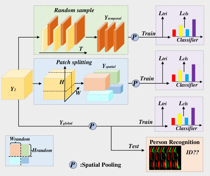
In this article, we will take the liberty of slightly reinterpreting the original approach proposed by the authors of S3CE-Net. While the original concept focused primarily on analyzing the spatiotemporal structure of an image, the nature of the signal being analyzed is different in the case of financial data. The market has no geometry — its structure is not visual but semantic. Here, the features constitute a vector of economic factors, where each coordinate carries its own context: price, volume, volatility, sentiment indicators, and structural liquidity metrics. And, most importantly, their interrelationships do not necessarily correlate with the proximity of their indices in this vector.

That is precisely why the direct application of spatial sampling, as in the classical STFS implementation for images, is not always justified. We cannot assume that adjacent elements in a feature vector have similar values or effects. In market data, neighborhood is defined by functional relationships. Price may be closely related to volume, but not at all to a technical indicator occupying the neighboring index in the data array.

For this reason, we use a reinterpreted sampling strategy similar to temporal sampling, but applied to the spatial (feature) axis. In other words, just as we select random time points in temporal sampling, here we will randomly select a subset of features to form a training sample for the model. This approach preserves the idea of randomness and generalization, but makes it relevant specifically to vector market data, where meaning — rather than location — is key.

Furthermore, unlike the original method — in which data not included in the sample are simply discarded — we will take a different approach. Not a single feature will be lost. From the remaining data, we will create alternative samples that will be used as supplementary contexts. This not only improves the effectiveness of training but also enhances the model’s robustness — it learns to view the market from different angles, as if analyzing it through a set of independent yet consistent observations.

As a result, five different representations of the analyzed data are generated:

• full (global), reflecting the overall market environment;
• 2 samples — temporal and feature-based, providing local focus for the model;
• 2 alternative samples that serve as additional sources for contextual learning.

We are also making changes to the way we generate the final forecast. In the classic STFS version for images, the features of the selected blocks are averaged, after which a single vector is formed. When applied to market data, this approach can smooth out important signals, causing subtle but significant impulses to be lost.

That is why we take a different approach: we generate a separate forecast for each of the samples obtained. In other words, the model does not combine information in advance, but analyzes each perspective separately. This makes it possible to evaluate signals in different contexts without losing the local significance of the data and while retaining the ability to distinguish weak but potentially important trends.

This approach is similar to the analytical style of a professional trader. An experienced trader never relies on a single indicator or a single time interval: they build several scenarios at once, compare them with one another, and use this basis to make a decision about the position. Similarly, our model learns to generate multiple forecasts based on the same information, viewing the market from different perspectives.

Now that the design concept for the STFS module has been defined and refined, it is time to move on to its practical implementation. The first step is to form five representations of the data being analyzed. To create all samples efficiently and in parallel, we use the OpenCL context, which allows us to process data arrays simultaneously and significantly speeds up the calculations.

The implementation is based on the STFS kernel, which creates subsamples using random masks of time steps and features. Each data point is checked for data validity, after which all necessary sample combinations are generated. This approach allows us to create both the main and alternative samples simultaneously, without waiting for sequential processing, which is critical when working with streaming market data.

__kernel void STFS(__global const float* inputs,
                   __global const float* mask_time,
                   __global const float* mask_spatial,
                   __global float* outputs
                  )
  {
   const size_t time_id = get_global_id(0);
   const size_t spat_id = get_global_id(1);
   const size_t head = get_local_id(2);
   const size_t total_times = get_global_size(0);
   const size_t total_spats = get_global_size(1);
   const size_t total_heads = get_local_size(2);
//---
   __local float temp[3];

For each position in the data stream, we define local and global identifiers by time, the spatial axis, and heads (heads), which are responsible for different types of samples.

In the first stage, offsets to the corresponding elements in the flat data buffers are determined.

   const int shift_in = RCtoFlat(time_id, spat_id, total_times, total_spats, 1);
   const int shift_out = RCtoFlat(time_id, spat_id, total_times, total_spats, head);

Next, the necessary values — including temporal and spatial masks — are retrieved from the global data buffers and used to filter the data.

To minimize the number of expensive global memory accesses, we distribute them among the workgroup's threads and store the values in a local memory array. As a result, each value is retrieved from the global buffer only once.

   switch(head)
     {
      case 0:
         temp[0] = IsNaNOrInf(inputs[shift_in], 0);
         break;
      case 1:
         temp[1] = IsNaNOrInf(mask_time[time_id], 0);
         break;
      case 2:
         temp[2] = IsNaNOrInf(mask_spatial[spat_id], 0);
         break;
     }
   BarrierLoc

The algorithm then creates separate subsamples. One is for the main temporal sample, the second for the alternative temporal sample, the third for the feature sample, and the fourth for the alternative feature sample.

   float out = temp[0];
   if(out != 0)
      switch(head)
        {
         case 1:
            out *= temp[1];
            break;
         case 2:
            out *= (1 - temp[1]);
            break;
         case 3:
            out *= temp[2];
            break;
         case 4:
            out *= (1 - temp[2]);
            break;
        }
//---
   outputs[shift_out] = IsNaNOrInf(out, 0);
  }

Each of these subsamples is stored in its own block of the results array for further processing by the model.

Thus, the kernel’s output is a complete set of five representations of the input data, ready for the subsequent generation of individual forecasts. This is a key aspect of the practical implementation of STFS: the model is able to learn simultaneously from different eyes of the market, viewing it both globally and locally, as well as through alternative lenses.

It is worth noting that the kernel algorithm for distributing error gradients is based on similar logic. We suggest leaving the implementation details of this mechanism for independent study. The complete code for the OpenCL program is included in the attachment.

The next step in our work is to build the STFS module within the main program, which will allow us to integrate all the concepts of sampling and forecast generation into a single architecture. To do this, a new CNeuronSTFS object is created, inheriting the basic capabilities of an OpenCL-enabled neuron from CNeuronBaseOCL.

class CNeuronSTFS    :  public   CNeuronBaseOCL
  {
protected:
   CNeuronBaseOCL    cMaskTime;
   CNeuronBaseOCL    cMaskSpatial;
   CNeuronBaseOCL    cConcatenated;
   CNeuronConvOCL    cSpatialDScale;
   CNeuronConvOCL    cTimeDScale;
   CNeuronTransposeVRCOCL caTranspose[2];
   CBufferFloat      cOne;
   //---
   virtual bool      STFS(CNeuronBaseOCL *NeuronOCL);
   virtual bool      STFSGrad(CNeuronBaseOCL *NeuronOCL);
   //---
   virtual bool      feedForward(CNeuronBaseOCL *NeuronOCL) override;
   virtual bool      updateInputWeights(CNeuronBaseOCL *NeuronOCL) override;
   virtual bool      calcInputGradients(CNeuronBaseOCL *NeuronOCL) override;

public:
                     CNeuronSTFS(void) {};
                    ~CNeuronSTFS(void) {};
   //---
   virtual bool      Init(uint numOutputs, uint myIndex, COpenCLMy *open_cl,
                          uint chanels_in, uint chanels_out, uint units_in, uint units_out,
                          ENUM_OPTIMIZATION optimization_type, uint batch);
   //---
   virtual int       Type(void)   override const   {  return defNeuronSTFS;   }
   //--- methods for working with files
   virtual bool      Save(int const file_handle) override;
   virtual bool      Load(int const file_handle) override;
   //---
   virtual void      SetOpenCL(COpenCLMy *obj) override;
   virtual void      SetActivationFunction(ENUM_ACTIVATION value) override;
   //---
   virtual bool      WeightsUpdate(CNeuronBaseOCL *source, float tau) override;
  };

The class structure reflects the key components of STFS: separate objects for temporal and feature masks (cMaskTime, cMaskSpatial), a tensor for merging representations (cConcatenated), and specialized convolutional and transpose layers (cSpatialDScale, cTimeDScale, caTranspose[2]) that ensure correct projection of spatiotemporal data. Together, all these elements form a platform that enables the model to account for various aspects of market information simultaneously and generate five forecast values derived from different representations.

All internal components of the CNeuronSTFS class are declared statically, allowing the constructor and destructor to be left empty. The object is created and initialized entirely within the Init method. This approach simplifies memory management and ensures predictable initialization of all parts of the module.

bool CNeuronSTFS::Init(uint numOutputs, uint myIndex, COpenCLMy *open_cl,
                       uint chanels_in, uint chanels_out, uint units_in, uint units_out,
                       ENUM_OPTIMIZATION optimization_type, uint batch)
  {
   if(!CNeuronBaseOCL::Init(numOutputs, myIndex, open_cl, chanels_out * units_out, optimization_type, batch))
      return false;
   activation = None;

The Init method performs sequential configuration of each internal component of the STFS module. First, the base initialization of the parent class is called, after which no activation is set on the main object.

It is particularly important to note here that the absence of an activation function at the module level is a prerequisite for the algorithm to function correctly. The authors of the S3CE-Net framework recommend using the STFS module only during the training phase. In production deployment, when the system generates forecasts in real time, only the complete data representation is used, without creating subsamples. Therefore, as will be shown below, the module returns only the forecast based on the complete representation, while all intermediate subsamples serve solely to strengthen the training process and build a more robust and accurate model. However, within the module, a parallel subsample training process is built, and to propagate gradients correctly across all components of the module, the raw error is required, without any adjustments for the derivative of the activation function.

At the same time, for flexibility depending on the user's needs, activation may still be used functionally, but it is moved to the last data projection object. It is there, when obtaining the final forecast, that a nonlinear transformation can be applied if required for a specific model operating scenario.

But let's return to the initialization algorithm. Next, masks for temporal sampling and feature sampling are created and configured. Each one is assigned its own index.

   int index = 0;
   if(!cMaskTime.Init(0, index, OpenCL, units_in, optimization, iBatch))
      return false;
   cMaskTime.SetActivationFunction(None);
   index++;
   if(!cMaskSpatial.Init(0, index, OpenCL, chanels_in, optimization, iBatch))
      return false;
   cMaskSpatial.SetActivationFunction(None);

The representation concatenation object is formed by taking into account all features and the sequence length, multiplied by the number of samples, thereby providing the basis for the subsequent forecast.

   index++;
   if(!cConcatenated.Init(0, index, OpenCL, chanels_in * units_in * 5, optimization, iBatch))
      return false;
   cConcatenated.SetActivationFunction(None);

After that, the projection block is initialized; it consists of convolutional layers for projecting the spatial and temporal components (cSpatialDScale, cTimeDScale), which are assigned the appropriate activation functions for correct scaling of the output signals.

   if(!cSpatialDScale.Init(0, index, OpenCL, chanels_in, chanels_in, chanels_out, units_in, 5, optimization, iBatch))
      return false;
   cSpatialDScale.SetActivationFunction(SoftPlus);
   index++;
   if(!cTimeDScale.Init(0, index, OpenCL, units_in, units_in, units_out, chanels_out, 5, optimization, iBatch))
      return false;
   cTimeDScale.SetActivationFunction(TANH);

The initialization is completed by transposition objects, which ensure consistent data transformation between different representations.

   index++;
   if(!caTranspose[0].Init(0, index, OpenCL, 5, units_in, chanels_out, optimization, iBatch))
      return false;
   if(!caTranspose[1].Init(0, index, OpenCL, 5, chanels_out, units_out, optimization, iBatch))
      return false;

The cOne buffer is used only in the error-gradient distribution algorithm and makes it possible to obtain copies of the data for all projections.

   if(!cOne.BufferInit(5, 1) ||
      !cOne.BufferCreate(OpenCL))
      return false;
//---
   return true;
  }

All components are configured to perform parallel computations on the OpenCL context side, ensuring high performance when processing arrays of market data.

The forward-pass algorithm is implemented in the feedForward method. Its task is to pass the data step by step through all the module components in order to obtain a ready-to-use representation for the forecast.

bool CNeuronSTFS::feedForward(CNeuronBaseOCL *NeuronOCL)
  {
   if(!STFS(NeuronOCL))
      return false;

First, the STFS method is called, creating five data representations: the complete representation, two samples, and two alternative samples. In it, unlike the familiar methods for queuing kernels for execution, the masks of the temporal steps and the analyzed features are sampled first. Only after the preparatory work has been completed is control passed to the corresponding kernel.

After that, the data passes through a convolutional layer for projecting spatial features, allowing the model to identify local structures and relationships between features in different representations.

   if(!cSpatialDScale.FeedForward(cConcatenated.AsObject()))
      return false;

Next, a tensor transformation is performed, ensuring correct conversion between the spatial and temporal representations.

   if(!caTranspose[0].FeedForward(cSpatialDScale.AsObject()))
      return false;

After that, the temporal projection convolution layer processes the data along the time axis, capturing market dynamics and identifying significant temporal patterns.

   if(!cTimeDScale.FeedForward(caTranspose[0].AsObject()))
      return false;

The second transpose layer restores the data to its original representation.

   if(!caTranspose[1].FeedForward(cTimeDScale.AsObject()))
      return false;

In the final stage, we extract only the data from the global representation, as the framework’s authors recommend for production deployment.

   if(!DeConcat(Output, caTranspose[1].getPrevOutput(), caTranspose[1].getOutput(),
                               Neurons(), caTranspose[1].Neurons() - Neurons(), 1))
      return false;
//---
   return true;
  }

Thus, the feedForward method ensures a smooth flow of data through the entire STFS module, laying the groundwork for subsequent error calculations, weight updates, and the generation of a final prediction based on a complete representation of the data.

Once the model has generated predicted values, the error-correction stage begins — backpropagation of gradients. The calcInputGradients method is responsible for distributing the error among all components of the STFS module in accordance with their influence on the final result.

bool CNeuronSTFS::calcInputGradients(CNeuronBaseOCL *NeuronOCL)
  {
   if(!NeuronOCL)
      return false;

It is important to note here that the STFS module can be used both at the output of a model and within a more complex architecture. In such cases, the input to backpropagation is not actual values, but an error passed from subsequent network components.

At the same time, different data projections — global, temporal, feature-based, and alternative samples — have different errors. To train each projection correctly, it is preferable to have target values rather than deviations. To obtain these target values, the module’s prediction results are summed with the incoming error, forming a tensor that can be used to train individual projections correctly.

That is precisely why the absence of an activation function at the module's output becomes critically important. Any nonlinear transformation would distort this process, and the network would lose its ability to correctly distribute errors and generate accurate target values for each projection.

   if(!SumAndNormilize(Output, Gradient, PrevOutput, 1, false, 0, 0, 0, 1))
      return false;
   if(!MatMul(GetPointer(cOne), PrevOutput, caTranspose[1].getGradient(), cOne.Total(), 1, Neurons(), 1, false))
      return false;

We multiply the resulting tensor of target values by a vector of ones, which gives us the required number of copies. At this point, we determine the error for each of the representations.

   float error = 1;
   if(!caTranspose[1].calcOutputGradients(caTranspose[1].getGradient(), error))
      return false;

Next, the gradients are propagated through the data projection block to the representation-concatenation tensor, carefully accounting for each element's contribution to the overall prediction.

   if(!cTimeDScale.CalcHiddenGradients(caTranspose[1].AsObject()))
      return false;
   if(!caTranspose[0].CalcHiddenGradients(cTimeDScale.AsObject()))
      return false;
   if(!cSpatialDScale.CalcHiddenGradients(caTranspose[0].AsObject()))
      return false;
   if(!cConcatenated.CalcHiddenGradients(cSpatialDScale.AsObject()))
      return false;

Special attention is given to STFSGrad — a wrapper function for the kernel of the same name, which aggregates errors within the STFS module from all subsamples and passes them to the original data.

   if(!STFSGrad(NeuronOCL))
      return false;
//---
   return true;
  }

It is precisely thanks to this mechanism that the model learns to identify and distinguish between global and local market patterns, thereby developing a robust and accurate forecasting model.

In practical terms, for a trader, this means that every element of the module, from subsamples to convolutional blocks, receives feedback on its significance for the final forecast, which improves the quality of training and enables the model to effectively handle noisy and volatile market data.

The complete code for the class and all of its methods is provided in the attachment.

Model Architecture

Now that all the key modules of the framework have been implemented, we move on to the next stage — describing the model architecture. Following the approach of the authors of S3CE-Net, we use the Environment State Encoder model from SEW-ResNeXt, which has proven effective at extracting meaningful features from streaming data.

Within this architecture, we introduce SSAM blocks that provide selective attention to the most informative features and their combinations. This approach allows the network to focus on key market signals while minimizing the impact of noise and random fluctuations, which is particularly important for highly volatile financial data.

To avoid overloading the article and to keep it readable, we do not include the full Encoder diagram. Details of the architecture are available in the attachment to the article, where each layer and block is described in detail. Readers can review the targeted changes to the architecture and the complete structure on their own.

It should be noted in particular that the STFS module is used exclusively during the training phase. In live deployment, when the model generates real-time forecasts, subsamples and separate data projections are unnecessary, and generating them only increases the load on system resources. To use computing resources efficiently, we have moved STFS into a separate model that is used only for training.

The model begins by creating the input data layer, which corresponds to the features being analyzed and the observation window.

//--- STFS
   stfs.Clear();
//--- Input layer
   if(!(descr = new CLayerDescription()))
      return false;
   descr.type = defNeuronBaseOCL;
   descr.count = (window * count);
   descr.activation = None;
   descr.optimization = ADAM;
   if(!stfs.Add(descr))
     {
      delete descr;
      return false;
     }

The next step is to add an STFS layer, where the channel and unit parameters for the input and output are specified. This layer performs a key function: it forms five data subsamples and calculates predictions for each one using the specified TANH activation function. It is this layer that enables parallel training across different market projections, thereby enhancing the model's robustness and its ability to identify meaningful signals.

//--- layer 1
   if(!(descr = new CLayerDescription()))
      return false;
   descr.type = defNeuronSTFS;
     {
      uint temp[] = {window,              // Channels In
                     BarDescr             // Channels Out
                    };
      if(ArrayCopy(descr.windows, temp) < (int)temp.Size())
         return false;
     }
     {
      uint temp[] = {count,               // Units In
                     NForecast            // Units Out
                    };
      if(ArrayCopy(descr.units, temp) < (int)temp.Size())
         return false;
     }
   descr.activation = TANH;
   descr.optimization = ADAM;
   if(!stfs.Add(descr))
     {
      delete descr;
      return false;
     }

The configuration concludes with a BatchNorm layer, which normalizes the output of the STFS block, maintaining training stability and preventing excessive gradient bias. In this case, this layer performs another important function: it learns the distribution of the target data and adds it to the predicted values generated by the STFS module.

//--- layer 2
   if(!(descr = new CLayerDescription()))
      return false;
   descr.type = defNeuronBatchNormOCL;
   descr.count = NForecast*BarDescr;
   descr.batch = BatchSize;
   descr.activation = None;
   descr.optimization = ADAM;
   if(!stfs.Add(descr))
     {
      delete descr;
      return false;
     }

Separating STFS into a standalone model allows for the separation of training and production use, reducing the load on the real-time system while fully preserving the benefits of parallel training across different market projections.

As for the architecture of the Actor and Critic models, it has been carried over entirely from our previous work. This makes it possible to retain time-tested solutions for generating actions and evaluating their quality. It also makes it possible to integrate new components without compromising training stability. The result is a full-fledged model that combines both traditional approaches to managing a market strategy and modern methods for identifying significant features and making robust forecasts.

Testing

We have completed a major effort to integrate all the key components of the framework, and now it is time to evaluate the effectiveness of the solutions we have implemented. But first, the strategy must be trained and thoroughly tested using historical and simulated data, much like honing the skills of an experienced trader and verifying the algorithm’s ability to perform under a wide variety of market conditions.

We will conduct the first stage — offline training — using historical data for the EURUSD currency pair on the H1 timeframe for the period from January 2024 to June 2025. This period served as a sort of training ground. The model learned to recognize historical patterns, understand price dynamics and trading volumes, identify relationships between key features, and use them in forecasts. Thanks to the STFS module, it simultaneously mastered global and local data representations, forming five different projections, which improved the accuracy and robustness of the forecasts. It could be said that the model developed trader’s intuition, combined with the mathematical rigor of data analysis.

The next stage — online fine-tuning in the MetaTrader 5 Strategy Tester — enabled the model to work with real-time data streams. Here, it mastered the dynamics of a live market, learned to maintain stability amid market noise, adjust its actions in low-liquidity conditions, and react instantly to sharp price spikes. SSAM blocks kept the focus on the most informative features, even when the data were unstable.

The final test was conducted using data from July through September 2025, which were entirely new and had not been used previously. All parameters obtained in the previous stages were loaded without modification, which ensured a fair assessment of the model's generalization ability. The results confirm that a step-by-step approach to training and adaptation, using STFS and SSAM, enables the model to analyze the market and generate forecasts of key market features that traders can rely on when making actual trading decisions.

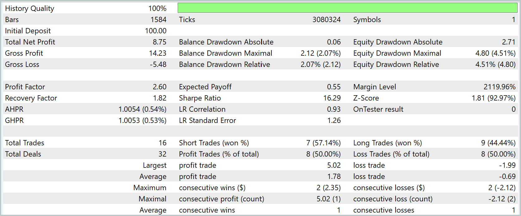
The results of the model testing demonstrate high stability and accuracy in the forecasts. The account balance showed steady growth from an initial deposit of USD 100 to USD 108.75, while equity smoothly tracked the balance, indicating that the forecast allocation and risk management mechanism was working correctly.

The maximum balance drawdown was only 2.07%, while the maximum equity drawdown was 4.51%, indicating a low level of risk and the strategy's resilience even amid market fluctuations. The overall profit factor is 2.60, which confirms the model's ability to effectively select profitable signals.

In terms of trade structure, 8 out of 16 trades were profitable, representing a 50% success rate, and the average profitable trade was 1.78, while the average loss was limited to 0.69, demonstrating a good balance between return and risk. The largest profit on a single trade reached 5.02, while the largest loss was limited to 1.99, which also confirms the model's prudence in capital management.

The model combining SSAM and STFS demonstrated modest, low-profile capital growth with a small drawdown and a good risk-reward ratio. The result is promising, but so far statistically limited. Before moving the strategy into live trading, more extensive tests and stress tests must be conducted to confirm the stability of its behavior over long and challenging market periods.

Conclusion

We went all the way from an idea to a working tool, doing it as if we were assembling a precise clockwork mechanism — carefully, step by step, and with attention to detail.

Using MQL5, we implemented the key components of S3CE-Net:

• implemented SSAM into the SEW-ResNeXt encoder,
• adapted STFS for a market feature vector,
• prepared an OpenCL kernel for the parallel generation of five representations.

The key engineering idea is the separation of modes. STFS works effectively, but its place is during training. In production, we keep only the global representation. This conserves resources and ensures predictable behavior. A practical detail that is important to keep in mind: the absence of activation within the module is not a matter of preference, but a requirement for correctly forming target tensors and propagating gradients between projections.

Tests conducted on EURUSD H1 for July–September 2025 showed promising results. The model takes a conservative approach. All of this provides a solid foundation, but it does not lock the strategy in for life.

What traders need to understand: current metrics are encouraging, but the sample size is small. High results based on a small sample can be misleading. Our task now is not to celebrate victory, but to test its robustness.

Links

• S3CE-Net: Spike-guided Spatiotemporal Semantic Coupling and Expansion Network for Long Sequence Event Re-Identification
• Other articles in this series

Software used in this article

#	Name	Type	Description
1	Study.mq5	Expert Advisor (EA)	EA for offline model training
2	StudyOnline.mq5	Expert Advisor (EA)	EA for online model training
3	Test.mq5	Expert Advisor (EA)	EA for model testing
4	Trajectory.mqh	Class Library	Structure for describing the system state and model architecture
5	NeuroNet.mqh	Class Library	Class library for building a neural network
6	NeuroNet.cl	Library	Code library for the OpenCL program