Implementation of the Gaussian Mixture Model in MQL5
 47
 0

Introduction
The Gaussian mixture model (GMM) is one of the most prominent classical examples of unsupervised learning. This is a parametric probabilistic model that assumes the observed data are generated by a weighted sum of several Gaussian distributions.
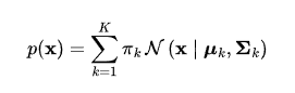
where:
- πk — the mixing coefficient of the kth mixture component (∑πk = 1),
- μk — the mean vector of the kth component,
- Σk — the covariance matrix of the kth component,
- N — the multivariate normal density.
Unlike classical clustering algorithms (such as k-means), GMM does not simply divide the data into groups, but rather models the probabilistic structure of the data. As a result, each point can belong to several clusters at once to varying degrees.
Real-world data do not always follow a single normal distribution. They often form several groups (clusters) with different cluster centers, shapes, and orientations in space. As an example, Fig. 1 schematically shows three normal components in two-dimensional space.
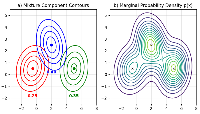
Fig. 1 A mixture of three normal distributions in two-dimensional space: a) density contours for each mixture component (the mixing coefficients are shown below each component), b) contours of the marginal probability density p(x) of the mixture distribution
It would be difficult to describe such a data structure using a single distribution, whereas a Gaussian mixture handles this task quite well.
As of today, there is no publicly available implementation of the Gaussian mixture model in MQL5. In this article, we will try to understand the model's structure, examine its underlying assumptions, and write a CGMM class in MQL5. This will allow you to perform clustering, multivariate probability density modeling, and data generation directly in MetaTrader 5, without having to constantly switch back to Python.
Key features of the implementation:
- Support for two training modes: MLE (maximum likelihood) and MAP (maximum a posteriori),
- Parameter initialization using K-Means++ (through integration with the Alglib library) or random initialization,
- Support for full covariance matrices, allowing any linear relationships between features to be captured,
- As in scikit-learn, methods are implemented for hard clustering (Predict), soft clustering (PredictProba), generating synthetic samples (Sample), computing the log-likelihood (ScoreSamples), and computing information criteria (AIC/BIC) to select the optimal number of clusters.
In the following sections, we will examine the mathematical foundation of the model, discuss the specifics of finding optimal parameters using the EM algorithm, and compare the results of our model's calculations with the reference implementation of GaussianMixture from the scikit-learn library.
A Mixture of Normal Distributions in Terms of Latent Variables
Suppose we have a sample of N independent and identically distributed observations {x, …, xN}, which can be represented as an N×D matrix X, where the nth row is the vector xn. Our goal is to describe this data using a Gaussian mixture model. The geometric shape and properties of such a mixture are entirely determined by the set of parameters θ = (π, μ, Σ):
- π = (π1, …, πk),
- μ = (μ1, …, μk),
- Σ = (Σ1, …, Σk).
To find these parameters, we must maximize the logarithm of the likelihood function:

Because of the sum over components inside the logarithm, parameter estimates cannot be obtained analytically. To overcome this difficulty, the GMM is expressed in terms of latent variables. This makes it possible to use the EM algorithm for training and to derive convenient analytical formulas for calculating the parameters. To do this, a K-dimensional binary variable z (a vector) with a one-hot representation is introduced, where znk = 1 if the nth observation is generated by the kth component, and 0 otherwise.
This representation of the model can be conveniently depicted as a probabilistic graph (Fig. 2).
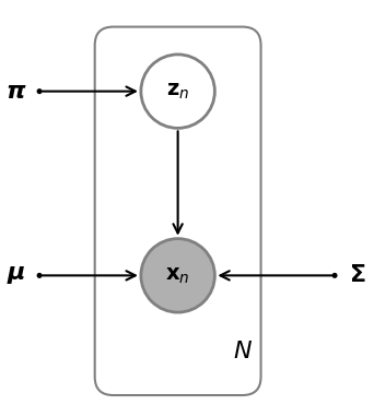
Fig. 2: A GMM represented as a graph for a set of N data points x with corresponding latent variables z
In the graph:
- The unshaded circle represents the latent variables zn,
- The black circle represents the observed variables xn,
- The model parameters are shown without circles (these are not random variables, but constants — albeit unknown ones).
The model assumes that all observations are independent and identically distributed (i.i.d.). This is clearly shown in the graph: each observation xn depends only on its own latent variable zn and is independent of the other observations.
Note:If the latent variable zn depends on its previous value zn-1, then such a model is called a hidden Markov model (HMM). You can read more about this model in my previous article, which discusses an important special case of the categorical (discrete) observation model.
The EM Algorithm for GMMs
The EM (expectation-maximization) algorithm is an iterative method for estimating parameters (MLE/MAP) in probabilistic models with latent variables. The main idea is to shift from optimizing a complex marginal likelihood (which cannot be differentiated directly using analytical methods) to maximizing the mathematical expectation of the logarithm of the joint distribution p(x, z), which significantly simplifies the calculations.
Let us consider the key distributions needed to understand how the EM algorithm works in the specific case of a GMM.
The prior distribution of the latent variable z:
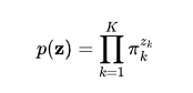
Conditional distribution of observations x given the latent variable z:
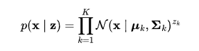
The joint distribution p(x, z) is defined by the expression p(x, z) = p(x|z)p(z), and the marginal distribution of x (which is what we call a GMM) is obtained by summing the joint distribution over all possible values of z:

Thus, we have arrived at an equivalent formulation of the Gaussian mixture, but now in terms of latent variables.
Another important distribution is given by the posterior probabilities that each point belongs to each component — the so-called responsibilities γ(znk). They can be found using Bayes' theorem:

Note that this is not an approximation: the distribution is computed exactly. Not all probabilistic models with latent states allow for such a simple calculation.
Now let's introduce the concept of a complete data set — {X, Z}. If we knew the true values of the latent variables, the complete-data log-likelihood would take a simple form:
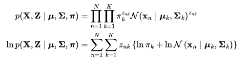
Please note that the sum is no longer inside the logarithm. Now it is much easier to calculate the derivatives with respect to the parameters. However, in practice, we do not know the values of the latent variables; we only have observations. To address this problem, we introduce an auxiliary function Q — the expectation of the complete-data log-likelihood with respect to the posterior distribution of the latent variables:

This is where the name of the first step of the EM algorithm comes from: "expectation" (mathematical expectation). Substituting the posterior probabilities into this formula, we get:

The auxiliary function Q is also called the evidence lower bound (ELBO), a lower bound on the marginal likelihood. It is shown that if we maximize this lower bound, we thereby also maximize the marginal likelihood.
In the particular case of a mixture model, we can differentiate the auxiliary function Q with respect to the model parameters to obtain convenient analytical formulas for updating these parameters in the M-step of the EM algorithm. It is not always possible to obtain such a simple M-step, which leads to various generalizations of the EM algorithm.
Thus, the EM algorithm consists of the following iterative steps:
- We choose the initial values for the parameters θ_old,
- E-step (Expectation) — we compute the posterior distribution of the latent variables,
- M-step (Maximization) — we maximize the Q function and obtain the updated parameters θ_new,
- We check the convergence of the log-likelihood function. If the convergence criterion is not met, then θ_new → θ_old, and we return to step 2.
Parameter Estimation by Maximum Likelihood (MLE)
The goal of the maximum likelihood method is to find model parameters θ = {π, μ, Σ} that maximize the likelihood of the observed data X. Mathematically, this problem boils down to maximizing the logarithm of the likelihood function.
After initializing the parameters and performing the E-step — computing the posterior probabilities γ(z) of the latent states — the algorithm proceeds to the M-step. Since the latent variables are discrete, these probabilities can conveniently be represented as a matrix (table of numbers). At this stage, parameter optimization becomes significantly easier because we work with the auxiliary function Q, whose derivatives are readily obtained in explicit analytical form.
Mean μk:
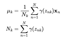
Here, Nk can be interpreted as the effective number of points assigned to cluster k. The mean μk of the kth Gaussian component is computed as the weighted mean of all data points. The weight for each point xn is determined by the posterior probability γ(znk) that component k is responsible for generating xn.
Covariance Σk:
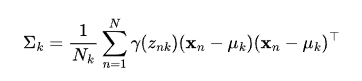
This formula is very similar to the classic covariance formula for a single normal distribution. However, in this case, each data point is again assigned a weight equal to its corresponding posterior probability, and the denominator is equal to the actual number of data points, Nk, associated with that component.
Mixing coefficients:
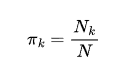
It is simply the ratio of the number of points assigned to the kth cluster to the total number of observations in the sample.
Maximum a Posteriori (MAP) Parameter Estimation
The maximum likelihood method often suffers from numerical instability, especially when the data are high-dimensional (D > 20) or the sample size is small. The main problem is the occurrence of degenerate or ill-conditioned covariance matrices.
A good solution is to switch from MLE to MAP estimation. In doing so, we remain within the framework of the same EM algorithm, but introduce prior distributions over the model parameters. Since the main instability arises specifically in the covariance matrices, the changes affect only the formula for updating them in the M-step. The E-step remains completely unchanged.
The normal-inverse-Wishart distribution (NIW) is used as the conjugate prior distribution for the mean and covariance. Because of prior conjugacy, there is no need to implement this complex probability density function. In practice, the entire Bayesian inference process boils down to a slightly modified MLE estimate at the M-step:
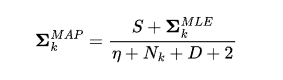
where
- S is the prior covariance of the normal-inverse-Wishart distribution. There are various ways to define it, but a reliable and adaptive option is to use a scaled diagonal matrix of variances of the original features:
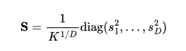
where sd is the empirical variance of feature d, calculated over the entire training sample.
- η (eta) is the parameter controlling the informativeness of the Wishart prior distribution. The least informative distribution is obtained by setting η = D + 2 (the larger η is, the stronger the regularization).
- Nk - the actual number of points assigned to cluster k,
- D - the dimension of the feature space,
- K is the number of components in the mixture.
CGMM Class
All of the mathematics described above is implemented as the CGMM class.
//+------------------------------------------------------------------+
//|                                                          GMM.mqh |
//|                                                           Eugene |
//|                                             https://www.mql5.com |
//+------------------------------------------------------------------+
#property copyright "Eugene"
#property link      "https://www.mql5.com"
#include <Math\Stat\Math.mqh>
#include <Math\Stat\Normal.mqh>
#include <Math\Alglib\alglib.mqh>

//--- type of model parameter estimation
enum ENUM_EM_MODE
  {
   MLE,
   MAP
  };

enum ENUM_INIT_MODE
  {
   KMEANS,  // Initialize cluster centers using K-Means++ (Alglib)
   RANDOM   // Initialize cluster centers with random numbers
  };

//+------------------------------------------------------------------+
//| Gaussian mixture model class                                     |
//+------------------------------------------------------------------+
class CGMM
  {
private:
   int               m_k;             // Number of clusters (K)
   ulong             m_dim;           // Feature dimensionality (D)
   bool              m_is_fitted;     // Flag indicating successful model training

   vector            m_pi;            // Cluster weights (priors) [K]
   matrix            m_mu;            // Cluster means [K][D]
   matrix            m_sigma[];       // Covariance matrices [K][D × D]

   ENUM_EM_MODE      m_estimate;      // Parameter estimation mode (MLE or MAP)
   ENUM_INIT_MODE    m_init_mode;     // Mean initialization mode (KMEANS or RANDOM)
   double            m_threshold;     // EM convergence threshold
   int               m_max_iters;     // Maximum number of iterations

   //--- Hyperparameters for MAP estimation
   matrix            m_S;             // Scale matrix of the prior distribution
   double            m_eta;           // Degrees of freedom of the prior distribution

   void              Initialize_parameters(const matrix &X);

   bool              e_step(const matrix &X, matrix &responsibilities);       // E-step of the EM algorithm
   bool              m_step(const matrix &X, const matrix &responsibilities); // M-step of the EM algorithm
   double            log_likelihood(const matrix &X); // The likelihood function for data X

public:

   vector            logliks; // likelihood history
   int               n_iter_; // the number of iterations performed by the EM algorithm

                     CGMM(int components, ENUM_EM_MODE estimate=MLE, double tol=1e-5, int max_iter=100,ENUM_INIT_MODE mode = KMEANS);
                    ~CGMM(void) {};

   // Methods for setting initial parameter values before training a model
   bool              SetInitialWeights(const vector &pi);
   bool              SetInitialMeans(const matrix &means);
   bool              SetInitialCovars(const matrix &covars[]);

   // Main methods
   bool              Fit(const matrix &X,bool verbose=false); // Training the model
   vector            Predict(const matrix &X);                // Cluster label vector [N]
   matrix            PredictProba(const matrix &X);           // [N x K] matrix of posterior cluster probabilities
   bool              Sample(const int n_samples, matrix &X, vector &labels); // Sample generation
   vector            ScoreSamples(const matrix &X);           // Vector of log probability densities [N]
   double            AIC(const matrix &X);                    // Akaike information criterion
   double            BIC(const matrix &X);                    // Bayesian information criterion

   // Getters for accessing model parameters
   vector            GetWeights(void)       { return m_pi; }
   matrix            GetMeans(void)         { return m_mu; }
   void              GetCovars(matrix &out_sigma[]);
  };
Main methods of the class:
- Fit(const matrix &X, bool verbose) — Trains the model on the data X using the EM algorithm. The 'verbose' parameter enables training progress (log-likelihood values) to be displayed,
- Predict(const matrix &X) — Performs hard clustering. Returns a vector of size N containing the cluster indices (from 0 to K-1) for each point,
- PredictProba(const matrix &X) — Performs soft clustering. Returns an N×K matrix containing the posterior probabilities of each point belonging to each component. The entries in each row sum to 1,
- ScoreSamples(const matrix &X) — Returns a vector of log marginal likelihood values, one for each observation,
- Sample(const int n_samples, matrix &X, vector &labels) — Generates synthetic data along with the true component labels,
- AIC(const matrix &X) and BIC(const matrix &X) are the Akaike and Bayesian information criteria. These are used to select the optimal number of clusters.
Before running the EM algorithm, you must specify the initial values for the parameters. Unless the user has specified them manually, the parameters are initialized automatically using the private method Initialize_parameters(const matrix &X).
//+------------------------------------------------------------------+
//| Initializing parameters                                          |
//+------------------------------------------------------------------+
void CGMM::Initialize_parameters(const matrix &X)
  {
   m_dim = X.Cols();

   // --- 1. Initializing weights (pi) ---
   //--- If the user has not specified the weights in advance, assign equal weights
   if(m_pi.Size() != (ulong)m_k)
     {
      m_pi.Init(m_k);
      m_pi.Fill(1.0 / m_k);
     }

   // --- 2. Initializing the means (mu) ---
   //--- If the cluster centers are not specified, we calculate them using K-Means++ or RANDOM
   if(m_mu.Rows() != (ulong)m_k || m_mu.Cols() != m_dim)
     {
      m_mu.Init((ulong)m_k, m_dim);

      if(m_init_mode == KMEANS)
        {
         CClusterizerState s;
         CKmeansReport rep;
         CMatrixDouble x;
         x = X;

         CAlglib::ClusterizerCreate(s);
         CAlglib::ClusterizerSetPoints(s, x, 2);        // 2 - Euclidean metric
         CAlglib::ClusterizerSetKMeansLimits(s, 1, 0);  // 1 restart, no limit on the number of iterations
         CAlglib::ClusterizerRunKMeans(s, m_k, rep);    // Run with m_k clusters

         if(rep.m_terminationtype > 0)
            m_mu = rep.m_c.ToMatrix(); // copied the cluster centers from K-Means++
         else
            m_init_mode = RANDOM; // If Alglib returns an error, switch to a random start
        }

      if(m_init_mode == RANDOM)
        {
         vector zero_mean = vector::Zeros(m_dim);
         matrix identity = matrix::Identity(m_dim, m_dim);
         CMVN::rnd(zero_mean, identity, m_k, m_mu); // Random centers
        }
     }

   // --- 3. Initializing covariance matrices (Sigma) ---
   // If the matrices are not specified, we use the feature variances computed over the entire sample
   if(ArraySize(m_sigma) != m_k)
     {
      ArrayResize(m_sigma, m_k);
      vector var_ = X.Var(0);
      matrix diag_variance;
      diag_variance.Diag(var_); // Create a diagonal matrix of variances
      for(int i = 0; i < m_k; i++)
         m_sigma[i] = diag_variance;
     }
  }
- Mixing coefficients are initialized uniformly,
- Cluster centers
This is the most important step, since the performance of the EM algorithm depends heavily on the proper selection of initial centers. The class supports two initialization modes:
- KMEANS (recommended) — cluster centers are calculated using the K-Means++ algorithm (Alglib library). This method significantly reduces the likelihood of getting stuck in a poor local maximum and speeds up model training.
- RANDOM — cluster centers are generated randomly from a multivariate normal distribution with a mean of zero and an identity covariance matrix.
- Covariance matrices are initialized identically for all components as diagonal matrices whose main diagonals contain the empirical variances of each feature, calculated over the entire sample X.
Model Training Method — Fit()
//+------------------------------------------------------------------+
//| Training the model                                               |
//+------------------------------------------------------------------+
bool CGMM::Fit(const matrix &X, bool verbose=false)
  {
   m_dim = X.Cols();
   m_is_fitted = false;

// --- Calculation of the hyperparameters S and eta when using MAP estimation ---
   if(m_estimate == MAP)
     {
      m_eta = (double)m_dim + 2.0;
      vector var = X.Var(0);
      m_S.Init(m_dim, m_dim);
      m_S.Fill(0.0);
      double k_correction = MathPow((double)m_k, 1.0 / (double)m_dim);
      for(ulong d = 0; d < m_dim; d++)
        {
         m_S[d, d] = var[d] / k_correction;
        }
     }

// --- Initializing parameters ---
   Initialize_parameters(X);

// --- Main loop of the EM algorithm ---
   logliks.Init(m_max_iters);
   logliks.Fill(0.0);
   double LL = log_likelihood(X);
   double prev_LL = 0.0;
   matrix responsibilities;
   int iter = 0;

   if(verbose)
      Print("   Iteration      LogLikelihood");

   while(iter < m_max_iters)
     {
      prev_LL = LL;
      if(!e_step(X, responsibilities)) // E-step
         return false;
      if(!m_step(X, responsibilities)) // M-step
         return false;

      LL = log_likelihood(X);
      logliks[iter] = LL;

      if(verbose)
         PrintFormat("     %6d   %15.5f", iter + 1, LL);

      iter++;
      n_iter_ = iter;

      if(MathAbs(LL / prev_LL - 1.0) < m_threshold)
        {
         if(verbose)
            PrintFormat("EM converged at %d iterations. Final Log-L value: %.5f", iter, LL);
         m_is_fitted = true;
         break;
        }
     }

   if(iter >= m_max_iters)
     {
      m_is_fitted = true;
      if(verbose)
         Print("Max number of EM iterations reached. Try different init parameters or increase max_iter.");
     }

   logliks.Resize(iter);

   return m_is_fitted;
  }
If the user selects the MAP parameter estimation mode, the hyperparameters S and eta are calculated automatically. After the parameters are initialized, the EM algorithm loop begins. The stopping criterion is checked: if the relative change in the log-likelihood falls below the threshold m_threshold (default: 1e-5), training ends. The E-step and M-step are implemented as separate functions.
//+------------------------------------------------------------------+
//| E-step of the EM algorithm                                       |
//+------------------------------------------------------------------+
bool CGMM::e_step(const matrix &X, matrix &responsibilities)
  {
   ulong N = X.Rows();
   responsibilities.Init(m_k, N); // Initialize the [K x N] matrix of posterior probabilities

// Step 1: Calculate the numerator in Bayes' formula for all K components (pi_k * PDF_k)
   for(int k = 0; k < m_k; k++)
     {
      vector pdf_k;
      if(!CMVN::pdf(X, m_mu.Row(k), m_sigma[k], pdf_k))
         return false;
      responsibilities.Row(pdf_k * m_pi[k], k);
     }

// Step 2: Sum down the columns to obtain the denominator of Bayes' formula for each point
   vector likelihood_old = responsibilities.Sum(0);
   likelihood_old.Clip(1e-300, DBL_MAX); // Division-by-zero protection for anomalous data points


// Step 3: Normalization
   for(int k = 0; k < m_k; k++)
      responsibilities.Row(responsibilities.Row(k) / likelihood_old, k);

   return true;
  }
The result of the E-step is a K × N responsibility matrix.
//+------------------------------------------------------------------+
//| M-step of the EM algorithm (M-step)                              |
//+------------------------------------------------------------------+
bool CGMM::m_step(const matrix &X, const matrix &responsibilities)
  {
   ulong N = X.Rows();

   for(int k = 0; k < m_k; k++)
     {
      vector resp_k = responsibilities.Row(k);
      double Nk = resp_k.Sum();

      //--- 1. Update the means
      m_mu.Row((resp_k @ X) / Nk, k);

      //--- 2. Calculate the weighted Sigma_k
      matrix W_dk(N, m_dim);
      for(ulong n = 0; n < N; n++)
         W_dk.Row((X.Row(n) - m_mu.Row(k))* MathSqrt(resp_k[n]), n);

      matrix Sigma_k = W_dk.Transpose() @ W_dk;

      //--- 3. Update the covariance matrices
      if(m_estimate == MLE)
        {
         m_sigma[k] = Sigma_k / Nk;
        }
      else
         if(m_estimate == MAP)
           {
            m_sigma[k] = (m_S + Sigma_k) / (m_eta + Nk + m_dim + 2.0);
           }

      //--- 4. Update the weights
      m_pi[k] = Nk / (double)N;
     }
   return true;
  }
The M-step yields updated model parameters.
Once training is successfully completed, the model is ready for use: you can estimate a data point's membership in a specific cluster, generate synthetic data, or evaluate the model's quality using the AIC/BIC criteria.
//+------------------------------------------------------------------+
//| Cluster prediction (hard clustering)                             |
//+------------------------------------------------------------------+
vector CGMM::Predict(const matrix &X)
  {
   vector labels(X.Rows());
   if(!m_is_fitted)
     {
      Print("Error: Model not trained!");
      return labels;
     }

   matrix resp = PredictProba(X); // probability matrix of size [N x K]
   labels = resp.ArgMax(1); // ArgMax(1) finds the index of the maximum value in each row

   return labels; // Return a vector of size [N] containing cluster numbers (0, 1, ... K-1)
  }

//+------------------------------------------------------------------+
//| Soft cluster prediction (soft clustering)                        |
//| Returns an [N x K] matrix, where:                                |
//| N - number of data points (rows)                                 |
//| K - number of clusters (probabilities for each component)        |
//+------------------------------------------------------------------+
matrix CGMM::PredictProba(const matrix &X)
  {
   matrix resp(X.Rows(),m_k);
   if(!m_is_fitted)
     {
      Print("Error: Model not trained!");
      return resp;
     }

   e_step(X, resp); // [K × N]

   return resp.Transpose(); //  [N × K]
  }

//+------------------------------------------------------------------+
//|Marginal likelihood                                               |
//+------------------------------------------------------------------+
double CGMM::log_likelihood(const matrix &X)
  {
  //--- Returns the log probability density for all data in sample X
   return ScoreSamples(X).Sum(); // Sum the vector of logarithms
  }

//+------------------------------------------------------------------+
//| Log-likelihood for each observation                              |
//+------------------------------------------------------------------+
vector CGMM::ScoreSamples(const matrix &X)
  {
   ulong N = X.Rows();
   matrix joint_density(m_k, N); // Joint density matrix p(x,z) of size [K x N]

//--- Step 1: Compute the joint density p(x,z) = p(x|z) * p(z)
   for(int k = 0; k < m_k; k++)
     {
      vector pdf_k;
      if(!CMVN::pdf(X, m_mu.Row(k), m_sigma[k], pdf_k))
         Print("Error in CMVN::pdf when calculating component ", k);

      //--- Multiply the conditional density p(x|z) by the prior probability of the latent state p(z)
      joint_density.Row(pdf_k * m_pi[k], k);
     }
//--- Step 2: Marginalization—sum over all states of z to obtain the marginal density p(x)
   vector likelihood = joint_density.Sum(0); // p(xn) = p(xn, z = 0) + p(xn, z = 1) + ⋯ + p(xn, z = K−1)

   likelihood.Clip(1e-300, DBL_MAX);// Guard against taking the logarithm of infinity for anomalous points

//--- Step 3: Take the natural logarithm of the probability density
   likelihood = MathLog(likelihood);

   return likelihood; // Return a vector of log-likelihoods of size [N]
  }
The marginal likelihood function is computed to monitor the convergence of the EM algorithm. For convenience and better compatibility with the scikit-learn library interface, the likelihood calculation has been split into two methods. ScoreSamples returns a vector of log probability densities, one for each observation, while the log_likelihood method returns the total marginal log-likelihood over the entire sample.
Implementation of a Multivariate Normal Distribution (CMVN Class)
Implementing a Gaussian mixture model would be technically impossible without methods for working with multivariate normal distributions (MVN). Since MQL5 does not yet have built-in tools for working with multivariate distributions, the CMVN class was created.
//+------------------------------------------------------------------+
//| Multivariate normal distribution                                 |
//+------------------------------------------------------------------+
class CMVN
  {
public:
   //+------------------------------------------------------------------+
   //| Generating random vectors (sample generation)                    |
   //| INPUT:                                                           |
   //|   Mu    - mean vector of size [d]                                |
   //|   Sigma - covariance matrix of size [d x d]                      |
   //|   N     - number of observations generated                       |
   //| OUTPUT:                                                          |
   //|   R     - matrix of generated data [N x d]                       |
   //+------------------------------------------------------------------+
   static bool       rnd(const vector &Mu, const matrix &Sigma, const int N, matrix &R)
     {
      ulong d = Sigma.Rows();

      if(N < 1 || d < 1)
         return false;
      if(Mu.Size() != d || Sigma.Cols() != d || !Sigma.IsSymmetric())
         return false;

      //--- Cholesky decomposition
      matrix L;
      if(!Sigma.FactorizationCholesky(L))
        {
         Print("mvnrnd error: Covariance matrix is not positive definite");
         return false;
        }

      int total_elements = (int)(N * d);
      double rand_array[];

      if(!MathRandomNormal(0.0, 1.0, total_elements, rand_array))
         return false;

      matrix Z(N, d);
      for(int n = 0; n < N; n++)
        {
         vector row_vec(d);
         for(ulong j = 0; j < d; j++)
           {
            row_vec[j] = rand_array[n * d + j];
           }
         Z.Row(row_vec, n);
        }

      //--- Linear transformation and addition of the mean
      R = Z @ L.Transpose();
      for(int n = 0; n < N; n++)
         R.Row(R.Row(n) + Mu, n);

      return true;
     }

   //+------------------------------------------------------------------+
   //| Calculation of the probability density function (PDF)            |
   //| INPUT:                                                           |
   //|   X     - a data matrix of size [N x D]                          |
   //|   Mu    - mean vector of size [D]                                |
   //|   Sigma - covariance matrix of size [D x D]                      |
   //| OUTPUT:                                                          |
   //|   y     - vector of probability densities of size [N]            |
   //+------------------------------------------------------------------+
   static bool       pdf(const matrix &X, const vector &Mu, const matrix &Sigma, vector &y)
     {
      ulong N = X.Rows();
      ulong D = X.Cols();

      // --- Dimension checks ---
      if(N < 1 || D < 1)
        {
         Print("mvnpdf error: X matrix is empty");
         return false;
        }
      if(Mu.Size() != D)
        {
         Print("mvnpdf error: The mean vector length must match the number of columns in X");
         return false;
        }
      if(Sigma.Rows() != D || Sigma.Cols() != D)
        {
         Print("mvnpdf error: Covariance matrix should be square and of D x D size");
         return false;
        }

      // --- Symmetry check ---
      if(!Sigma.IsSymmetric())
        {
         Print("mvnpdf error: Covariance matrix should be symmetric");
         return false;
        }

      // --- Cholesky decomposition
      matrix L; // Lower-triangular matrix L (Sigma = L * L^T)
      if(!Sigma.FactorizationCholesky(L))
        {
         Print("mvnpdf error: Covariance matrix should be positive definite");
         return false;
        }

      // --- Data centering (X0 = X - Mu)
      matrix X0(N, D);
      for(ulong n = 0; n < N; n++)
         X0.Row(X.Row(n) - Mu, n);

      // --- Solution of a triangular system of equations (LAPACK TRTRS)
      matrix B = X0.Transpose(); // Dimensions: D x N
      matrix X_sol;              // D x N solution

      if(!L.LinearEquationsSolutionTriangular(EQUATIONSFORM_N, B, X_sol))
        {
         Print("mvnpdf error: Failed to solve the triangular system of equations");
         return false;
        }

      // --- Calculate the logarithm of the square root of a determinant
      vector diagL = L.Diag();
      double logSqrtDetSigma = 0.0;
      logSqrtDetSigma =  MathLog(diagL).Sum();

      // --- Compute a quadratic form
      vector quadform = (X_sol * X_sol).Sum(0);

      //--- Final density calculation ---
      //--- Compute the vector of log densities
      vector logPdf = -0.5 * quadform - logSqrtDetSigma - (D * MathLog(2.0 * M_PI)) / 2.0;
      //--- Take the exponential of each element of the vector logPdf
      y = MathExp(logPdf);
      return true;
     }
  };
The class contains two functions required for the GMM to work:
- pdf — computes the probability density of a multivariate normal distribution,
- rnd — generates random vectors from a multivariate normal distribution.
When developing the CMVN class, the primary focus was on performance, since the probability density function is called multiple times at each iteration of the EM algorithm. To do this, methods from the high-performance linear algebra library OpenBLAS are used:
- FactorizationCholesky — performs a Cholesky decomposition of a covariance matrix and checks it for positive definiteness (analogous to LAPACK's POTRF),
- LinearEquationsSolutionTriangular — solution of triangular systems of linear equations (analogous to LAPACK's TRTRS) to accelerate the calculation of the quadratic form without explicitly computing the inverse matrix.
Comparison of Training Results with the scikit-learn Model
To verify the correctness of the CGMM class implementation, a comparison was performed with the GaussianMixture model from the scikit-learn library (Python).
The classic Old Faithful dataset — which contains data on geyser eruptions in Yellowstone National Park in the United States — was used as the test set. The dataset contains 272 observations and two variables:
- eruption duration (in minutes),
- Time until the next eruption (in minutes).
Fig. 3 clearly shows that the data consist of two distinct clusters.
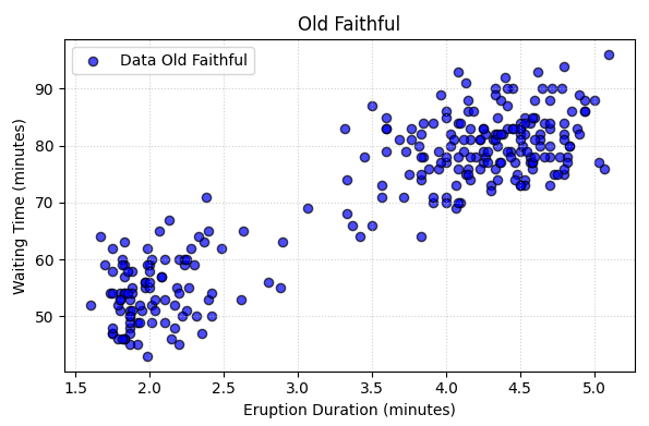
Fig. 3 Relationship between the time until the next eruption and the duration of the current eruption (Old Faithful dataset)
The data were loaded, standardized, and fed into a model with K = 2 components. Training was conducted in MLE mode.
//+------------------------------------------------------------------+
//|                                                     Learning.mq5 |
//|                                                           Eugene |
//|                                             https://www.mql5.com |
//+------------------------------------------------------------------+
#property copyright "Eugene"
#property link      "https://www.mql5.com"
#property version   "1.00"
#include <GMM\GMM.mqh>
#include <Graphics\Graphic.mqh>


//+------------------------------------------------------------------+
//| Script program start function                                    |
//+------------------------------------------------------------------+
void OnStart()
  {
// 1. Loading the Old Faithful dataset (272 observations, 2 features)
   matrix X;
   CSVtoMatrix("GMM/OldFaithful.csv",X);
   ulong N = X.Rows();
   ulong D = X.Cols();

// 2. Data normalization
   vector mean_ = X.Mean(0);
   vector std_ = X.Std(0);
   matrix X_norm(N, D);
   for(ulong i = 0; i < N; i++)
      X_norm.Row((X.Row(i) - mean_) / std_, i);

// 3. Creating the model
   int components = 2;
   CGMM gmm_model(components,MLE);
// CGMM gmm_model(components, MAP, 1e-5, 100);

// 4. Initializing parameters using setters
// --- Initial weights ---
   vector init_pi = {0.5, 0.5};
   gmm_model.SetInitialWeights(init_pi);

// --- Initial cluster means ---
   matrix init_means = {{-1.5, 1.5}, {1.5, -1.5}};
   gmm_model.SetInitialMeans(init_means);

// --- Initial covariance matrices (0.1 * Identity) ---
   matrix m = {{0.1, 0.0}, {0.0, 0.1}};
   matrix init_covars[2];
   init_covars[0] = m;
   init_covars[1] = m;
   gmm_model.SetInitialCovars(init_covars);

// 5. Starting training
   if(gmm_model.Fit(X_norm,true))
     {
      Print("=== The model has been successfully trained! ===");

      // 1. Weights after training
      vector final_pi = gmm_model.GetWeights();
      Print("Final weights (pi): ", final_pi);

      // 2. Means and covariance matrices
      matrix final_means = gmm_model.GetMeans();
      matrix final_covars[];
      gmm_model.GetCovars(final_covars);

      for(int k = 0; k < components; k++)
        {
         PrintFormat("--- Cluster %d ---", k);
         Print("Mean (mu): ", final_means.Row(k));
         Print("Covariance (Sigma):\n", final_covars[k]);
        }

      Print("------------------------------------------------");

      //--- Extract a subset containing the first 5 data points
      matrix first_five(5, D);
      for(ulong i=0; i<5; i++)
         first_five.Row(X_norm.Row(i), i);

      // --- Hard clustering
      vector predicted_labels = gmm_model.Predict(first_five);
      Print("Predicted clusters for the first 5 points:\n ", predicted_labels);

      // --- Soft clustering
      matrix predicted_probas = gmm_model.PredictProba(first_five);
      Print("Probability matrix [5 x 2] (rows - data, columns - cluster probabilities):\n", predicted_probas);

      vector score_samples = gmm_model.ScoreSamples(X_norm);
      //Print("Total log-likelihood (Total Log-L): ", score_samples.Sum());

      // --- Information criteria
      Print("================================================");
      Print("=== INFORMATION CRITERIA OF THE MODEL ===");

      double aic_value = gmm_model.AIC(X_norm);
      double bic_value = gmm_model.BIC(X_norm);

      PrintFormat("AIC (Akaike Information Criterion): %.5f", aic_value);
      PrintFormat("BIC (Bayesian Information Criterion): %.5f", bic_value);
      Print("================================================");
     }
   else
     {
      Print("Error: Failed to train GMM model");
     }
   VisualizeGMMTraining(gmm_model);
  }
//+------------------------------------------------------------------+
//| Visualization of the GMM learning curve                          |
//+------------------------------------------------------------------+
void VisualizeGMMTraining(CGMM &gmm_model)
  {

   int plotLimit = (int)gmm_model.logliks.Size();
   double x[], y_[];
   ArrayResize(x, plotLimit);
   ArrayResize(y_, plotLimit);

   for(int i = 0; i < plotLimit; i++)
     {
      x[i] = i;
      y_[i] = gmm_model.logliks[i];
     }
   ChartSetInteger(0, CHART_SHOW, false);
   CGraphic graphic;
   ulong width = ChartGetInteger(0, CHART_WIDTH_IN_PIXELS);
   ulong height = ChartGetInteger(0, CHART_HEIGHT_IN_PIXELS);
   graphic.Create(0, "GMM_Training_Plot", 0, 0, 0, int(width), int(height));
   CCurve *curve = graphic.CurveAdd(x, y_, ColorToARGB(clrDodgerBlue, 255), CURVE_LINES, "LogLikelihood");
   graphic.BackgroundMainColor(ColorToARGB(clrBlack, 255));
   graphic.BackgroundMainSize(24);
   graphic.BackgroundMain("GMM EM Training Progress");
   graphic.XAxis().Name("Iteration");
   graphic.XAxis().NameSize(18);
   graphic.YAxis().Name("Log Likelihood");
   graphic.YAxis().NameSize(18);
   graphic.CurvePlotAll();
   graphic.Update();
   Sleep(10 * 1000);
   ChartSetInteger(0, CHART_SHOW, true);
   graphic.Destroy();
   ChartRedraw(0);
  }
//+------------------------------------------------------------------+
After setting the initial parameters (in this example, they were set manually), we start training using the Fit() method. To log the marginal likelihood values during training, set the verbose argument to true.
Figure 4 shows the training results
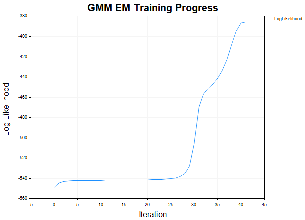
Fig. 4. Learning curve of the GMM for the Old Faithful data
After training, the script logs the following:
- optimized parameter values,
- the final value of the likelihood function,
- cluster labels for the first 5 points (Hard Clustering),
- a probability matrix for the first 5 points (Soft Clustering),
- the AIC/BIC information criterion values.
To verify that our class works correctly, we will compare the results we obtained with those from the scikit-learn reference library. To do this, a script named scikit.py was created, which used the same data, the same number of components, a similar initialization, and the same training settings.
import numpy as np
from sklearn.mixture import GaussianMixture
import matplotlib.pyplot as plt

# 1. Reading the Old Faithful dataset
file_path = r"C:\Program Files\MetaTrader 5\MQL5\Files\GMM\OldFaithful.csv"
X = np.genfromtxt(file_path, delimiter=',')

# 2. Data normalization
X_mean = X.mean(axis=0)
X_std = X.std(axis=0)
X_norm = (X - X_mean) / X_std

# 3. Initial parameters
init_pi = np.array([0.5, 0.5])
init_mu = np.array([[-1.5, 1.5], [1.5, -1.5]])
init_Sigma = np.array([np.identity(2) * 0.1, np.identity(2) * 0.1])

# 4. Configuring and training the scikit-learn GMM
gmm = GaussianMixture(
    n_components=2,
    covariance_type="full",
    tol=1e-5,
    max_iter=100,
    weights_init=init_pi,
    means_init=init_mu,
    precisions_init=np.linalg.inv(init_Sigma),  # Scikit requires precision matrices
    verbose=0
)

gmm.fit(X_norm)

# Convert the mean log-likelihood to the total log-likelihood
total_log_likelihood = gmm.score(X_norm) * X_norm.shape[0]

print(f"=== Scikit-Learn: EM converged in {gmm.n_iter_} iterations ===")
print("Final Log-L:", total_log_likelihood)
print("Final weights (pi):", gmm.weights_)

for i in range(2):
    print(f"\n--- Cluster {i} ---")
    print("Average (mu):", gmm.means_[i])
    print("Covariance (Sigma):\n", gmm.covariances_[i])

print("\n" + "-"*48)

# 5. Slice the first 5 points for prediction
first_five = X_norm[:5]

# Obtain hard labels (clusters 0 or 1)
predicted_labels = gmm.predict(first_five)
print("Predicted clusters for the first 5 points:")
print(predicted_labels)

# Obtain the probabilities (size [5 x 2])
predicted_probas = gmm.predict_proba(first_five)
print("\nProbability matrix [5 x 2] (rows - data, columns - clusters):")
print(np.round(predicted_probas, 10))

score_samples = gmm.score_samples(X_norm)
#print("score_samples:")
#print(score_samples)

# --- Information Criteria ---
print("\n" + "="*48)
print("=== MODEL INFORMATION CRITERIA  ===")

aic_value = gmm.aic(X_norm)
bic_value = gmm.bic(X_norm)

print(f"AIC (Akaike Information Criterion): {aic_value:.5f}")
print(f"BIC (Bayesian Information Criterion): {bic_value:.5f}")
print("="*48)

# ==============================================================================
# PLOT: Original data
# ==============================================================================
plt.figure(figsize=(6, 4))
plt.scatter(X[:, 0], X[:, 1], c='blue', s=35, alpha=0.7, edgecolors='k', label='Data Old Faithful')
plt.title("Old Faithful")
plt.xlabel('Eruption Duration (minutes)')
plt.ylabel('Waiting Time (minutes)')
plt.grid(True, linestyle=':', alpha=0.6)
plt.legend()
plt.tight_layout()
plt.show()

# ==============================================================================
# PLOT: Soft clustering (PredictProba)
# ==============================================================================
# We obtain the probabilities for the entire sample
all_probas = gmm.predict_proba(X_norm)

proba_cluster_1 = all_probas[:, 1]
plt.figure(figsize=(6, 4))
scatter = plt.scatter(X[:, 0], X[:, 1], c=proba_cluster_1, cmap='bwr', s=35, alpha=0.8, edgecolors='k')
plt.title("Soft Clustering of Old Faithful Dataset (PredictProba)")
plt.xlabel('Eruption Duration (minutes)')
plt.ylabel('Waiting Time (minutes)')
plt.grid(True, linestyle=':', alpha=0.6)

cbar = plt.colorbar(scatter)
cbar.set_label('Probability of Cluster 1', rotation=270, labelpad=15)

plt.tight_layout()
plt.show()
The model parameters, likelihood, predictions, and information criteria all agreed with those from the MQL5 implementation to 5–6 decimal places.
The results of soft data clustering using the PredictProba method are shown in Fig. 5
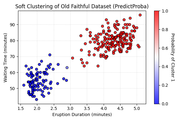
Fig. 5 Soft clustering using the PredictProba method
Sample Generation
A GMM is a generative model. Therefore, it can be used not only for clustering or estimating density, but also for generating new data. To do this, the CGMM class implements the Sample() method.
//+------------------------------------------------------------------+
//| Generating random samples (trajectories) from a trained GMM      |
//| INPUT:                                                           |
//|   n_samples - the number of data points to be generated          |
//| OUTPUT:                                                          |
//|   sample_X  - matrix of generated data  [n_samples x D]          |
//|   labels    - a vector of labels (cluster indices) [n_samples]   |
//+------------------------------------------------------------------+
bool CGMM::Sample(const int n_samples, matrix &sample_X, vector &labels)
  {
   if(n_samples <= 0)
     {
      Print("Error: Number of samples should exceed 0");
      return false;
     }

   int K = m_k;
   int D = (int)m_mu.Cols();

// --- Step 1: Select clusters for all N points  ---
   int cluster_indices[];
   ArrayResize(cluster_indices, K);
   for(int k = 0; k < K; k++)
      cluster_indices[k] = k;

   double pi[];
   VectorToArray(m_pi,pi);

   int z[];
   ArrayResize(z, n_samples);

   if(!MathSample(cluster_indices, pi, n_samples, true, z))
     {
      Print("Error : MathSample call failed");
      return false;
     }

   sample_X.Init(n_samples, D);
   labels.Init(n_samples);

   for(int s = 0; s < n_samples; s++)
      labels[s] = (double)z[s]; //--- Transfer the labels to the output vector

// --- Step 2: Generate data in batches for each cluster using mvnrnd
   for(int k = 0; k < K; k++)
     {
      //--- Count how many data points were assigned to the current cluster k
      int samples_in_cluster = 0;
      for(int s = 0; s < n_samples; s++)
        {
         if(z[s] == k)
            samples_in_cluster++;
        }

      //--- If there are data points for this cluster, generate them in a single batch
      if(samples_in_cluster > 0)
        {
         vector current_mu = m_mu.Row(k);
         matrix cluster_samples;

         if(!CMVN::rnd(current_mu, m_sigma[k], samples_in_cluster, cluster_samples))
           {
            PrintFormat("Error: mvnrnd failed to generate samples for cluster %d.", k);
            return false;
           }

         //--- Place the generated batch at its original indices
         ulong current_row_idx = 0;
         for(int s = 0; s < n_samples; s++)
           {
            if(z[s] == k)
              {
               sample_X.Row(cluster_samples.Row(current_row_idx), s);
               current_row_idx++;
              }
           }
        }
     }

   return true;
  }
The sampling process consists of two consecutive steps:
- Latent component selection: For each new observation, a mixture component is randomly selected according to the mixing coefficients π. This is done using the MathSample function from the standard statistics library.
- Batch coordinate generation: For each component, the number of points to be generated from it is calculated. Next, the CMVN::rnd() method is used to generate a batch of vectors from the corresponding multivariate normal distribution. The resulting points are then placed at their respective indices in the output matrix sample_X.
Figure 6 shows a sample of 1,000 data points generated using the parameters obtained by training the GMM on the Old Faithful dataset (Sample.mq5 script).
//+------------------------------------------------------------------+
//|                                                       Sample.mq5 |
//|                                                           Eugene |
//|                                             https://www.mql5.com |
//+------------------------------------------------------------------+
#property copyright "Eugene"
#property link      "https://www.mql5.com"
#property version   "1.00"
#include <GMM\GMM.mqh>
//+------------------------------------------------------------------+
//| Script program start function                                    |
//+------------------------------------------------------------------+
void OnStart()
  {
   // 1. Create a GMM object (2 components)
   CGMM gmm(2);

   // 2. Set the parameters
   vector init_pi = {0.35592792679548113, 0.6440720732045188};
   gmm.SetInitialWeights(init_pi);

   matrix init_means = {
      {-1.27384982, -1.20981836},
      {0.70395651,  0.66857136}
   };
   gmm.SetInitialMeans(init_means);

   matrix m0 = {{0.05337263, 0.02822063}, {0.02822063, 0.18303629}};
   matrix m1 = {{0.13083678, 0.06071860}, {0.06071860, 0.19563396}};
   matrix init_covars[2];
   init_covars[0] = m0;
   init_covars[1] = m1;
   gmm.SetInitialCovars(init_covars);

   // 3. Generate samples
   matrix sample_X;
   vector sample_z;
   if(gmm.Sample(1000, sample_X, sample_z))
     {
      Print("Sample successfully generated");
      MatrixToCSV("GMM_Samples.csv", sample_X);
      VectorToCSV("GMM_Labels.csv", sample_z);
     }
  }
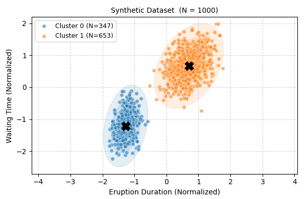
Fig. 6: A synthetic sample of 1,000 data points generated by the GMM
As shown in the figure, the synthetic data accurately reproduce the structure of the original Old Faithful dataset (two distinct clusters with characteristic shapes and orientations). Please note that the visualization is presented on a standardized scale.
Selecting the Optimal Number of Mixture Components (Model Selection)
When working with real data, a researcher generally does not know in advance how many latent states or mixture components are present in the data. Increasing the number of components almost always increases the value of the likelihood function, since the model gains more degrees of freedom and can fit the noise. This leads to overfitting.
To strike a reasonable balance between the quality of a model's fit and its complexity, the following information criteria are used:
- AIC (Akaike Information Criterion) penalizes a model in proportion to the number of free parameters,
- BIC (Bayesian Information Criterion) imposes a stricter penalty that also takes sample size into account.
The optimal number of components is the one that minimizes the corresponding information criterion value.
The ModelSelection.mq5 script demonstrates the process of selecting the optimal number of components (from 1 to 5) using the Old Faithful dataset.
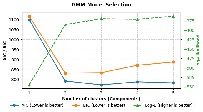
Fig. 7: Log-likelihood, AIC, and BIC as functions of the number of model components
As shown in Fig. 7:
- The log-likelihood increases monotonically as the number of components increases,
- BIC reaches its minimum at two components,
- AIC reaches its minimum at three components.
This behavior is typical: BIC tends to favor more parsimonious models, while AIC may allow for slightly more complex ones. The final selection of the optimal number of components in a GMM is largely a heuristic process based on expert judgment, rather than a rigorous automated procedure. AIC and BIC are useful heuristics, not absolute criteria for truth. In practice, it is recommended to consider the results of both criteria simultaneously and analyze the model's behavior for different numbers of clusters.
To run the scikit.py script, you will need a Python interpreter and the standard suite of statistical packages. For instructions on how to install them, see the article Python + MetaTrader 5: A Quick Research Loop for Data, Features, and Prototypes.
After installing the packages, place the scikit.py file in a folder (for example, Scripts/GMM).
Run the script using MetaEditor:
- In MetaEditor, click File → Open and select the scikit.py file from the GMM folder,
- After opening the file, press the F7 key (or click the "Compile" button on the toolbar),
- The calculation results should appear in the Journal tab.
Conclusion
In this article, we have provided a detailed analysis of the theory and practical implementation of the Gaussian mixture model in MQL5.
Key advantages of the GMM:
- Soft clustering — the model outputs not just a cluster number, but the probabilities of each data point belonging to all components of the mixture, which allows for more well-founded conclusions,
- Flexibility — thanks to full covariance matrices, the model is capable of describing clusters of any shape, size, and orientation in space,
- High-quality initialization — by default, the K-Means++ algorithm (Alglib) is used, which significantly speeds up the convergence of the EM algorithm and reduces the likelihood of getting stuck in unfavorable local maxima,
- Generative capability — a trained model can be used to generate new synthetic data whose statistical properties are similar to those of the original data,
- Statistical validity — built-in support for the AIC and BIC information criteria allows for the objective selection of the optimal number of components and helps prevent overfitting.
- Numerical stability — support for MAP estimation with a normal-inverse-Wishart distribution as the prior significantly improves training stability for small samples and high-dimensional data.
It is particularly important that the CGMM class produces results that are fully comparable to those of scikit-learn's GaussianMixture, while running directly within MetaTrader 5 without any external dependencies. This allows you to retrain the model whenever you deem it necessary, rather than locking in the same set of parameters for every possible scenario.
The Gaussian mixture model represents an important step from simple clustering toward a true probabilistic approach, and this tool is now available to every MQL5 developer.
Programs used in this article
| # | Name | Type | Description |
|---|---|---|---|
| 1 | GMM.mqh | Include file | Contains a Gaussian mixture model class and a multivariate normal distribution class |
| 2 | Learning.mq5 | Script | Example of model training |
| 3 | Sample.mq5 | Script | Example of sample generation |
| 4 | ModelSelection.mq5 | Script | Example of selecting the number of model components |
| 5 | scikit.py | Script | An example of training the GaussianMixture model from the sklearn library |
| 6 | OldFaithful.csv | CSV | Data in CSV format |
| 7 | MQL5.zip | Archive | All of the files listed above can be found in the archive |
Translated from Russian by MetaQuotes Ltd.
Original article: https://www.mql5.com/ru/articles/23279
Warning: All rights to these materials are reserved by MetaQuotes Ltd. Copying or reprinting of these materials in whole or in part is prohibited.
This article was written by a user of the site and reflects their personal views. MetaQuotes Ltd is not responsible for the accuracy of the information presented, nor for any consequences resulting from the use of the solutions, strategies or recommendations described.