Markov Chains in Trading and Price Forecasting

Introduction

In today's financial market, traders are constantly looking for new tools to forecast prices and make informed decisions, and they have an ever-growing number of such tools at their disposal — from SMA to AI (apparently, you have not seen the movie The Terminator). In this article, we will discuss one undeservedly forgotten tool — Markov chains.

It is no secret that many approaches and strategies considered classic no longer work in modern trading. And there is nothing surprising about that: the market is evolving every day, and no one knows where this evolution will lead. In today's market, anything can happen — noise, a cycle, a trend, or all of them at once. And this is where every trader faces the key question: what can we expect from the market, at least tomorrow?

In this article, we will explore the predictive capabilities of Markov chains in trading and look at examples of their practical use. According to the creator of these chains, their use can reduce the uncertainty that arises in market conditions, while models built on them make it possible to create trading algorithms and make decisions based on the probability of specific events occurring. This could provide an impetus for developing new strategies that take statistically significant patterns in market behavior into account.

Fundamentals of Markov Chains

A Markov chain is a mathematical model that is successfully applied in a wide variety of fields. It was proposed by A. Markov in 1906, in his article "On the Limit Distribution of a Class of Correlated Random Variables," in which he studied the statistical behavior of a chain of correlated random events.

The essence of the model is that it allows us to predict the probability of transitioning from one state to another. Thus, using a Markov chain, we can describe the properties of a given process and generate new sequences that resemble that process. These chains can be used to simulate and analyze processes occurring in the market.

Markov chains are based on two key factors: state and transition probability. The states of the chain can be described using both quantitative and qualitative variables. For example, if a value in a time series falls within the range of 10–20, then it is in state 1. Or, if the time series is increasing, its state is "U." The type of states depends on the process under study, and their number may be fixed or, in some cases, determined by the researcher.

Another important property of chains is that they have no memory. This means that the next state depends on the current state and is not related to the history in any way. Because of this property, Markov chains allow us to model nonstationary financial time series — their properties change over time. This is important during periods of high volatility, when trends can change rapidly and it is difficult to predict how the price will behave.

Now let's take a look at how to build Markov chains and how they can be applied in practice.

Simple Markov Chain

To start, let's build a simple Markov chain. For example, let's say it identifies market phases. We will define these phases as follows: we will consider a trend to be a situation in which the price moves a certain number of points over a specified number of bars. Otherwise, the market is flat. In total, we will have 3 market states. We will assign a unique index to each state:

• 0 – downtrend,
• 1 – flat market,
• 2 – uptrend.

First, we need to create a transition probability matrix. Its size depends on the number of states, and in this case, it will be 3×3. Let's initialize the values in this matrix to zero and populate it with historical data. Let the market state on this bar be denoted by the index i, and on the next bar by the index j. In that case, we need to increase the value in the cell with those indices by 1.

All that is left for us to do is convert the collected statistics into probabilities. To do this, we first need to find the sum of all the elements in a single row, and then divide each element in that row by the sum we found. As a result, we will obtain a probability matrix describing the market's transition from one state to another. This matrix might look like this.

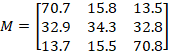
From this matrix, we can see that if the market is in the flat market state, then in the next step it may move to any other state with almost equal probabilities. The probabilities of the trend continuing are quite high.

This matrix can be used to predict future states. Let's add a forecast matrix. Initially, it is equal to the transition matrix and contains forecasts for one step ahead.

To find the forecast two steps ahead, we need to multiply these matrices together.

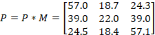
By continuing these multiplications, we can find forecasts for any number of steps ahead. However, it is important to keep in mind that as the number of steps increases, the practical value of the forecast decreases. Each new step smooths the probabilities, and eventually they will become equal to one another. In other words, regardless of the market's current state, after a certain number of steps, it will end up in any possible state with equal probability.

Matrix multiplication is necessary when analyzing the properties of the resulting chain. In practice, it is more convenient to proceed as follows. Take the row of the matrix that corresponds to the current state and convert it into a row vector. By multiplying this vector by the matrix, you will obtain a new vector containing the prediction for the next step.

We have examined a Markov chain based on qualitative variables. Now let's see how we can construct a Markov chain based on quantitative data.

Making the Chain More Complex

Forecasting is one of the most important tasks a trader faces. Successfully forecasting a future price value can yield significant profit. Let's see how we can build such a forecast using Markov chains.

There are many different ways to describe the market state, but they are all related in one way or another to price dynamics. In this case, we will use the price change over a specified number of bars.

First, let's see what values these differences can take. Intuition suggests that large increments should occur less frequently than small ones. But it's better to see it for ourselves.

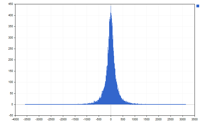
Now we need to specify the number of states and how they are defined. As an example, I selected 9 states, each of which appears approximately the same number of times in the historical data. Next, we can build the chain and begin making predictions. The latest state is known to us and is described by the difference.

Knowing the current state, we can estimate the next one and the probability that it will be exactly that state. Based on these probabilities, we can make a forecast of price movements. For each state, we know its minimum and maximum values. Let's take their average as the expected value.

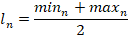
Now we can begin forecasting the price. Let's take a step forward. Then we will obtain differences of the following form:

Based on these differences, we can easily estimate future price values and their probabilities. And the forecast on the chart might look like this.

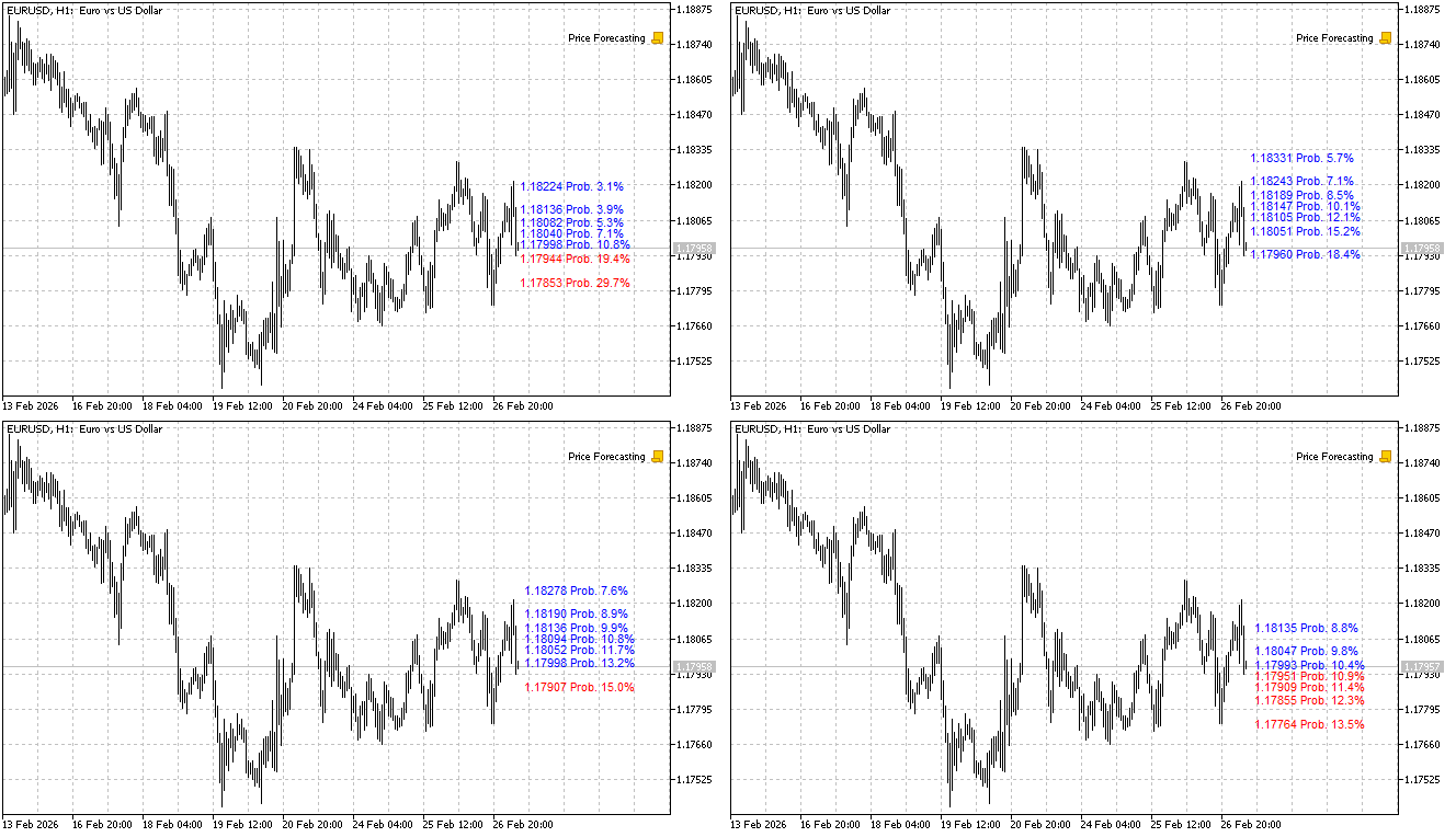
Now let's discuss some practical issues in applying Markov chains. Some processes may have a limited number of states. For example, if we roll a die, we will have 6 states. For other processes, the number of states can be arbitrary. In this case, it is necessary to first study the process and only then make assumptions about the number of possible states and the methods for determining them.

When constructing a Markov chain based on price differences, we used a probability measure to determine the states. But we could have done it differently. For example, we could calculate the expected value and standard deviation and define the boundaries of the chain's states as follows:

In this case, the number of states is unknown in advance, and the probabilities of their occurrence will vary.

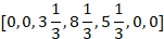
Some changes can also be made when calculating the transition matrix. First, we collect statistics on the number of chain transitions from one state to another. Let's assume that one of the rows of the matrix looks like this:

The first assumption we can make is that the next transition could be any of those we have already observed. Since there are only 3 such transitions, we need to increase the nonzero values by 1/3.

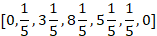
Our next assumption is that some very rare transitions may not have been included in our statistics. It is reasonable to assume that the chain may transition to the states closest to those already observed. In that case, the number of possible transitions will reach 5, and we need to increase the corresponding values by 1/5.

That way, we will exercise reasonable caution and be prepared for the arrival of a "black swan."

Knowing the market's history is a good thing, but no one knows what the future holds for the market. A situation that seems impossible to us today could happen tomorrow. In order to account for this possibility, we can assume that the chain can transition to any possible state.

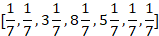
Such a Markov chain will be ready for the arrival of a flock of "black swans" of every possible color. However, this approach is acceptable only when the number of states is not very large.

Price Forecasting

A Markov chain is a fairly flexible tool that can be applied in a wide variety of ways. Let's try to predict the most likely price movement.

First, we need to determine what kind of price movement we will consider significant. For example, suppose the threshold for such a movement is 20 points. Next, we need to find the highest and lowest price values in the historical data. Now we can calculate the number of states in the future chain:

Let's prepare a transition matrix of the appropriate size and start filling it in. The current price state can be calculated using the following formula:

All other calculations remain the same. We will use the most likely price state at each step as our forecast. To calculate the price value, we can take the average value of this state:

An indicator based on this chain looks like this on the chart.

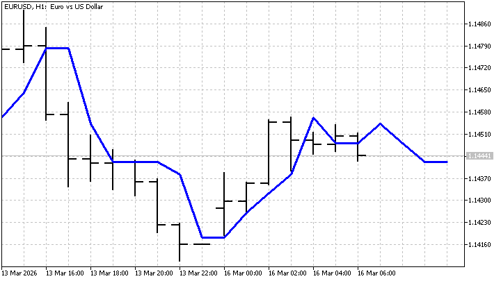
This is the simplest way to make a forecast. We will try using a more complex version. One of the advantages of Markov chains is that they can be used to examine different possible future price paths.

Let's say you have decided to open a position. Using a Markov chain, you can estimate future price values and the probabilities that they will be exactly those values. Based on this information, you can assess the potential outcomes and risks, which will help you decide whether it makes sense to open a position.

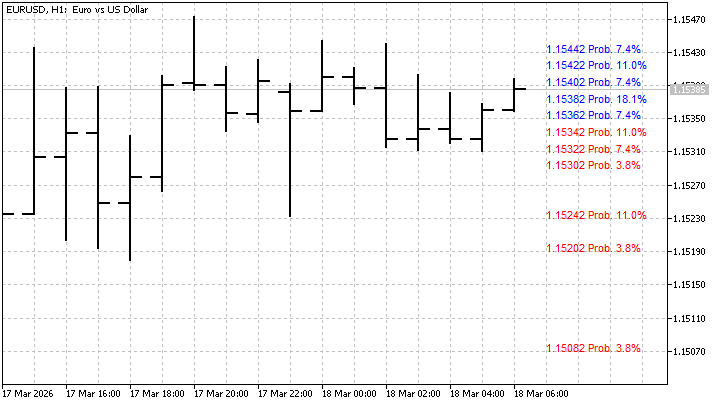
Forecasts can also be based on indicators. For example, you can use EMA values instead of prices. This indicator smooths the time series while preserving information about the trend. Therefore, a forecast based on this indicator will be smoother.

Markov Chains and Capital Management

Markov chains can be used for more than just market forecasting. They can also be used in other areas related to trading. Let's take a look at how they can be used for capital management.

Expected value is one of the most important metrics of a trading strategy. You can use it to estimate the average profit per trade. Another statistic that interests us right now is the Z-score. Using this metric, a trader can assess whether a sequence of wins and losses is random.

These characteristics provide insight into the trading strategy as a whole. Now let's see how we can characterize a trading system using a Markov chain. The chain will have only two states: loss and win. Each new trade refines the values in the transition matrix, and, as usual, we can use this matrix to predict future outcomes.

For example, I simulated 100 trades. The probability of winning is 64%, and the expected value is 21 points. It would seem that after so many trades, there should not be any surprises. However, that is not the case.

If the last trade in the sequence is a loss, the probability of winning the next trade increases to 68%, and the expected value rises to 30 points. However, after a winning trade, the probability of a win and the expected value drop to 61% and 14 points. In other words, the chain advises us to increase the position size after a loss and decrease it after a win.

But the main advantage of the Markov chain is that it processes information in real time. It is still unclear what the overall outcome of trading will be, but decisions must be made right here and now. And of course, using the chain, we can predict possible outcomes several steps ahead.

Conclusion

In this article, we explored some ways to apply Markov chains in trading and saw that this mathematical model is quite effective. They do not provide clear-cut answers, but they can reveal possible scenarios for the future, and in a market environment, such information can be worth its weight in gold.

Markov chains have their drawbacks. For example, memorylessness does not allow the influence of the past to be taken into account (this shortcoming can be overcome). However, their advantages far outweigh any disadvantages. The main advantage of Markov chains is their ability to process information and learn from new data. Using them in trading helps reduce market-related uncertainty. This can improve the effectiveness of trading strategies and help achieve more stable results.

The following programs were used to write this article:

Name	Type	Features
Simple Markov Chain	script	The script generates a forecast based on a simple trend. The forecast results are displayed in the "Experts" tab. iPeriod — the trend period. Level — the trend level Forecast — the number of forecast steps.
Price Forecasting	script	The script forecasts price levels using a differencing approach. The results are saved in the Files folder. iPeriod — the trend period. State — the number of states of the chain. FontSize - font size.
Price Forecast	indicator	The indicator forecasts the most likely price movement. Step - price change increment. Forecast — the number of forecast steps.
Price Level Forecasting	indicator	The indicator displays projected price levels.
Money Management	script	The script calculates the win probability and expected value. The forecast results are displayed in the "Experts" tab. Probability - the probability of winning for the simulated trades. Trades - number of simulated trades. Forward - the number of steps for the forecast. SL, TP - stop levels used to calculate the expected value.