Nonlinear OHLC Features Derived from Elliptic Curves

You are building a model to predict the direction of the next daily EURUSD candlestick and face a practical problem: the classic set of TA features (returns, MA/RSI, volatility, candlestick proportions) yields limited improvement, while attempts to make it more complex lead to overfitting and poor portability across market regimes. A new feature source is needed, deterministically computed from OHLC data, that provides a nonlinear representation of price, integrates easily into the existing ML pipeline, and is validated by a fair temporal split using AUC.

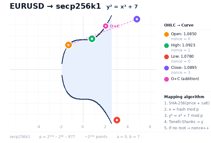
In this article, we address exactly this task. The method is simple to formulate: we map OHLC values to points on the secp256k1 elliptic curve using SHA-256 + try-and-increment, extract metadata from the points and the mapping process (nonce, x bits, Open+Close/High+Low group arithmetic), combine them with classic TA features, and test their added value in CatBoost on a time-based split. An experiment on 2,000 EURUSD D1 candlesticks yields a measurable result (test AUC = 0.6508), while the signal proves to be regime-dependent — the key practical conclusion of the article.

Next:

• intuition for elliptic curves,
• price mapping code,
• feature engineering,
• CatBoost results on 2,000 EURUSD D1 candlesticks.

What elliptic curves are and why secp256k1

An elliptic curve is the set of points (x, y) that satisfy the equation:

y² ≡ x³ + ax + b (mod p)

Bitcoin uses the secp256k1 curve, where a = 0 and b = 7. All calculations are performed modulo a very large prime number, p = 2²⁵⁶ – 2³² – 977. The curve contains about 2²⁵⁶ points — more than the number of atoms in the universe.

Parameter	Value	Description
Curve	secp256k1	Used in Bitcoin
Equation	y² = x³ + 7	Coefficients a=0, b=7
Field	Fp, p = 2²⁵⁶ – 2³² – 977	A huge prime number
Order	~2²⁵⁶	Number of points on the curve
Mapping	SHA-256 + try-and-increment	Price → x → check y²

Why is this interesting for trading?

Two operations are defined on an elliptic curve: point addition and scalar multiplication. When we map the Open and Close prices to points on the curve and add them, we get a third point — the combined “candlestick fingerprint” in a nonlinear space. To find a point on the curve, x³ + 7 must be a quadratic residue modulo p. So let's use a try-and-increment approach: we hash the price and check the candidate x. If the validation fails, we increase the nonce and try again. This nonce turns out to be an informative feature in and of itself.

Mapping: From Price to a Point on the Curve

Step 1. Price hashing. We take the price (Float64) and concatenate it with the salt (price type + candlestick index) and the nonce. We run it through SHA-256. We get a 256-bit number.

Step 2. Obtaining x. We take the hash modulo p: x = hash mod p. A candidate for the x-coordinate.

Step 3. Checking y². We compute y² = x³ + 7 mod p. If it is a quadratic residue, we find y using the Tonelli–Shanks algorithm.

Step 4. Try-and-increment. If not, we increase the nonce and repeat. Number of attempts (nonce) — metadata about the "complexity" of the mapping.

P = 0xFFFFFFFFFFFFFFFFFFFFFFFFFFFFFFFFFFFFFFFFFFFFFFFFFFFFFFFEFFFFFC2F
A, B = 0, 7

def price_to_curve_point(value, salt="eurusd"):
    """
    Mapping numerical price value for the secp256k1 elliptic curve point.
    Method: SHA-256 hashing + try-and-increment
    """
    value_str = f"{salt}:{value:.10f}"
    for nonce in range(256):
        data = f"{value_str}:{nonce}".encode('utf-8')
        h = hashlib.sha256(data).digest()
        x = int.from_bytes(h, 'big') % P
        y_sq = (pow(x, 3, P) + B) % P
        y = tonelli_shanks(y_sq, P)
        if y is not None:
            if y % 2 != 0:
                y = P - y  # canonical form (even y)
            return (x, y, nonce)
    return None

Note that the salt includes the price type (open, high, low, close) and the candlestick index. This ensures that identical prices in different candlesticks correspond to different points on the curve.

The Tonelli–Shanks Algorithm

def tonelli_shanks(n, p):
    """Calculating square root of n mod p"""
    if pow(n, (p - 1) // 2, p) != 1:
        return None  # no square root — not a quadratic residue

    Q, S = p - 1, 0
    while Q % 2 == 0:
        Q //= 2
        S += 1

    if S == 1:
        return pow(n, (p + 1) // 4, p)

    z = 2
    while pow(z, (p - 1) // 2, p) != p - 1:
        z += 1

    M, c = S, pow(z, Q, p)
    t, R = pow(n, Q, p), pow(n, (Q + 1) // 2, p)

    while True:
        if t == 1:
            return R
        i, temp = 0, t
        while temp != 1:
            temp = pow(temp, 2, p)
            i += 1
        b = pow(c, 1 << (M - i - 1), p)
        M, c = i, pow(b, 2, p)
        t, R = (t * c) % p, (R * b) % p

Arithmetic on a Curve: Point Addition

This is a key operation that makes it possible to combine the Open and Close points:

def extended_gcd(a, b):
    if a == 0: return b, 0, 1
    g, x, y = extended_gcd(b % a, a)
    return g, y - (b // a) * x, x

def mod_inverse(a, m=P):
    if a < 0: a = a % m
    g, x, _ = extended_gcd(a, m)
    return x % m

def point_add(p1, p2):
    """Summing two points on secp256k1"""
    if p1 is None: return p2
    if p2 is None: return p1
    x1, y1 = p1
    x2, y2 = p2
    
    if x1 == x2 and y1 != y2:
        return None  # the point at infinity
    
    if x1 == x2:
        # Point Doubling
        lam = (3 * x1 * x1) * mod_inverse(2 * y1) % P
    else:
        lam = (y2 - y1) * mod_inverse(x2 - x1) % P
    
    x3 = (lam * lam - x1 - x2) % P
    y3 = (lam * (x1 - x3) - y1) % P
    return (x3, y3)

On 2,000 EURUSD D1 candlesticks: 54% of prices are mapped on the first attempt (nonce=0), 24% on the second attempt, and 14% on the third attempt. This is consistent with the theoretical expectation: approximately half of the elements of Fp are quadratic residues.

Feature Engineering: Extracting Features from the Curve

We developed 96 features in 5 groups. Of these, 65 are features derived from the elliptic curve (EC), and 31 are classic TA features. All features are calculated for 4 lookback windows: 5, 10, 20, and 50 bars.

Group	Number of features	Type	Examples
Nonce features	~28	EC	nonce_mean_50, nonce_entropy_20
x-coordinate	~25	EC	x_slope_20, x_high, x_byte0
Point arithmetic	~12	EC	oc_x, hl_x, dx_norm
Classical TA	~25	TA	return_1, sharpe_20, rsi
Cross features	~6	EC×TA	nonce_x_ret_5, x_x_vol_20

Nonce entropy:

# Nonce entropy over the lookback window
from collections import Counter

def nonce_entropy(nonces_window):
    cnt = Counter(nonces_window)
    total = sum(cnt.values())
    return -sum(
        (v/total) * np.log2(v/total + 1e-10) 
        for v in cnt.values()
    )

x_slope — the trend of the x-coordinates on the curve.

# x_slope — the trend of the x-coordinates on the curve
def compute_x_slope(x_bits_array, lookback):
    """Linear trend of normalized x coordinates"""
    if len(x_bits_array) < 3:
        return 0
    x_idx = np.arange(len(x_bits_array))
    slope = np.polyfit(x_idx, x_bits_array, 1)[0]
    return slope

Point arithmetic — a combined candlestick fingerprint.

# A combined candlestick fingerprint on the curve
pt_open = price_to_curve_point(candle['open'], f"open:{i}")
pt_close = price_to_curve_point(candle['close'], f"close:{i}")

# Point addition on the curve: Open + Close → new point
combined = point_add(
    (pt_open[0], pt_open[1]),
    (pt_close[0], pt_close[1])
)

# x-coordinate of the combined point → feature
oc_x = int.from_bytes(
    combined[0].to_bytes(32, 'big')[:8], 'big'
) / (2**64)

Connecting to MetaTrader 5

To work with real data, we use the MetaTrader 5 library for Python:

import MetaTrader5 as mt5
from datetime import datetime

def load_mt5_data(symbol="EURUSD", timeframe="D1", n=2000):
    """Loading data via MetaTrader 5"""
    if not mt5.initialize():
        print(f"MT5 init failed: {mt5.last_error()}")
        return None
    
    tf_map = {
        'M1': mt5.TIMEFRAME_M1, 'M5': mt5.TIMEFRAME_M5,
        'M15': mt5.TIMEFRAME_M15, 'H1': mt5.TIMEFRAME_H1,
        'H4': mt5.TIMEFRAME_H4, 'D1': mt5.TIMEFRAME_D1,
        'W1': mt5.TIMEFRAME_W1, 'MN1': mt5.TIMEFRAME_MN1,
    }
    
    rates = mt5.copy_rates_from_pos(
        symbol, tf_map[timeframe], 0, n
    )
    mt5.shutdown()
    
    if rates is None or len(rates) == 0:
        print(f"No data for {symbol}")
        return None
    
    return [{
        'date': datetime.fromtimestamp(r['time']).strftime('%Y-%m-%d'),
        'open': round(float(r['open']), 5),
        'high': round(float(r['high']), 5),
        'low': round(float(r['low']), 5),
        'close': round(float(r['close']), 5),
    } for r in rates]

The script automatically attempts to connect to MetaTrader 5. If the terminal is not running, it uses data generated by a regime-switching model for testing.

CatBoost: Training and Results

We trained three CatBoost ensembles, each consisting of 3 models with different hyperparameters (depth 3–6, lr 0.01–0.05). Target variable: the direction of the next candlestick (1 = bullish, 0 = bearish). Time-based split: 70/15/15.

from catboost import CatBoostClassifier, Pool

# Three configurations for the ensemble
configs = [
    {'depth': 4, 'lr': 0.02, 'l2': 3, 'iters': 1000, 'sub': 0.8, 'rsm': 0.8},
    {'depth': 6, 'lr': 0.01, 'l2': 1, 'iters': 1500, 'sub': 0.7, 'rsm': 0.7},
    {'depth': 3, 'lr': 0.05, 'l2': 5, 'iters': 800,  'sub': 0.9, 'rsm': 0.9},
]

models = []
for cfg in configs:
    model = CatBoostClassifier(
        iterations=cfg['iters'],
        depth=cfg['depth'],
        learning_rate=cfg['lr'],
        l2_leaf_reg=cfg['l2'],
        subsample=cfg['sub'],
        rsm=cfg['rsm'],
        random_seed=42,
        verbose=0,
        eval_metric='AUC',
        early_stopping_rounds=100,
        use_best_model=True,
        bootstrap_type='Bernoulli',
    )
    model.fit(
        Pool(X_train, y_train, feature_names=names),
        eval_set=Pool(X_val, y_val, feature_names=names)
    )
    models.append(model)

# Ensemble: probability averaging
ensemble_probs = np.mean(
    [m.predict_proba(X_test)[:, 1] for m in models], 
    axis=0
)

Results for 2000 EURUSD D1 candlesticks:

Model	Val Acc	Val AUC	Test Acc	Test AUC	CV AUC
Full (EC + TA)	59.25%	0.5902	60.07%	0.6508	0.507 ± 0.02
TA baseline	56.51%	0.5719	60.07%	0.5992	0.536 ± 0.03
EC only	51.37%	0.5690	60.41%	0.5957	0.524 ± 0.04

Top-10 Feature Importance:

#	Feature	Importance	Type	Description
1	return_1	6.13%	TA	Daily return
2	ma_ratio_50	4.09%	TA	Price / MA(50)
3	x_slope_20	3.00%	EC	Trend of x-bits over 20 bars
4	x_slope_50	2.95%	EC	Trend of x-bits over 50 bars
5	sharpe_20	2.87%	TA	Sharpe Ratio (20 bars)
6	x_slope_5	2.50%	EC	Trend of x-bits over 5 bars
7	x_high	2.46%	EC	Most significant bits of the x-coordinate
8	oc_x	2.23%	EC	x-coordinate of Open+Close
9	ret_std_5	1.85%	TA	Volatility (5 bars)
10	x_x_vol_5	1.83%	EC×TA	x_bits × volatility

Analysis: Why EC Features Work

We analyze not individual points, but the statistics of the point distribution within the window. A single hash is noise. One hundred hashes in a row constitute a distribution, and this distribution has structure. Different price regimes (trend, sideways market, high/low volatility) generate different distributions of points on the curve. It is precisely this meta-information that CatBoost captures.

There is also a second source of signal—the nonce. The number of attempts to find a quadratic residue depends directly on the value of x³ + 7 mod p, which is determined deterministically by the price.

• x_slope — speed along the curve

x_slope — the linear trend of the normalized x-coordinates over a window of 5, 20, or 50 bars. High positions of x_slope in the importance ranking indicate that the nonlinear curve space does indeed add useful information. Trending markets and sideways markets produce different trajectories on the curve, even after hashing. All three scales — x_slope_5, x_slope_20, and x_slope_50 — made it into the top 10.

• nonce_entropy — market regime indicator

The nonce is deterministic for a fixed salt, so the distribution of nonces within the window reflects the properties of the price set rather than random noise. nonce_entropy_20 — 12th place (1.81%); it is particularly useful in combination with ATR: periods of high volatility with high nonce_entropy represent one regime, while high volatility with low nonce_entropy represents another.

• oc_x — a nonlinear "candlestick fingerprint"

Two candlesticks with the same body (Close – Open = 50 pips) but different absolute price levels will yield completely different oc_x points. A group operation on an elliptic curve is a form of nonlinear feature engineering built into the curve’s mathematical structure. oc_x ranks 8th (2.23%) — surpassing RSI and ATR.

• Cross-features: Synergy Between EC and TA

x_x_vol_5 (x_bits × volatility over 5 bars) — 10th place (1.83%). EC features and TA features reinforce each other. EC features are not a replacement for classical technical analysis, but rather an extension of it into a new space.

Honest Assessment

Cross-validation (5-fold) shows: Full CV AUC = 0.507 versus TA CV AUC = 0.536. On average across all market regimes, the full model does not outperform the TA baseline. Test set: AUC 0.6508 vs. 0.5992. A 5.2 percentage point gap is significant.

A likely explanation is the regime-dependence of the EC signal. EC features are stronger during trending phases and weaker in sideways markets. Below is a practical scenario for switching between models:

• determine the current market regime (trend/sideways market) using ADX, VIX, or a Hidden Markov Model
• In trending phases, use the full model (EC + TA)
• In sideways phases, fall back to the TA baseline
• Determine the switching threshold using a validation set

Other Curves

• Curve25519 (Ed25519) is a Montgomery curve used in Signal, SSH, and TLS 1.3. Equation: y² = x³ + 486662x² + x.
• BN254 is a pairing-friendly curve used in Ethereum (EIP-197). Supports bilinear pairings.
• BLS12-381 is a modern pairing-friendly curve used in Ethereum 2.0, Zcash, and Filecoin.

The idea behind the multi-curve ensemble: we map EURUSD to secp256k1, Curve25519, and BLS12-381 simultaneously, extract features from each curve, and combine them into a single matrix.

Pairing-based features

On pairing-friendly curves (BN254, BLS12-381), it is possible to compute the bilinear pairing e(P, Q). Pairing is bilinear: e(aP, bQ) = e(P, Q)^(ab). This creates a natural way to encode products of prices. Implementation using the py_ecc library for Python.

Market Regime Detector

• ADX: if ADX > 25, it is a trending market — use EC + TA; if ADX < 20, it is a sideways market — use TA only.
• Hidden Markov Model: 2–3 states based on historical returns, each with its own set of weights for EC and TA.
• Self-detection: nonce_entropy as a built-in detector — if the entropy is above the threshold, the EC features are informative.

Multi-instrument analysis

Map EURUSD, GBPUSD, USDJPY, and XAUUSD to a single curve and analyze the relative positions of the points. The “centroid” of the portfolio on the curve — the sequential point addition of all instruments — may reflect systemic risk or the general direction of the foreign exchange market.

Online Learning

MetaTrader 5 ↔ Python integration via WebSocket: The EA receives a new bar → sends OHLC data → Python calculates EC features → CatBoost makes a forecast → the result is returned to the EA. Calculating EC features takes about 2 ms per candlestick, which is fast enough even for M1.

Quantum Extensions

Points on the curve serve as inputs for quantum kernel methods. Each point (x, y) is encoded as a qubit state: Ry(x/P × π) × Rz(y/P × π). On NISQ hardware — approximately 20–30 qubits, i.e., a window of 10–15 candlesticks. The Qiskit and PennyLane libraries support quantum kernel methods with classical SVM/CatBoost on the output side.

What We Proved

An experiment involving 2000 EURUSD D1 candlesticks yielded three specific, measurable results. First: The secp256k1 elliptic curve, developed to secure cryptocurrency transactions, contains a structure that is useful for forecasting financial time series. This is not a trivial fact — SHA-256, with its avalanche effect, should have destroyed any connection with the original price. It turned out that the statistics of the distribution of points over the window retain information about the price regime even after hashing.

Second result: the x_slope feature — the trend of the normalized x-coordinates of the points on the curve — ranked 3rd and 4th in terms of importance, ahead of the RSI, ATR, and most classical indicators. This feature has no equivalent in traditional technical analysis. This means that the curve adds a fundamentally new dimension to the feature space, rather than simply duplicating existing signals.

Third result: oc_x — the x-coordinate of the sum of the Open and Close points on the curve — proved to be more informative than simply Close – Open. Two candlesticks with identical 50-pip bodies but at different price levels yield different oc_x values. Elliptic curve group arithmetic automatically takes the absolute price level into account, which no standard candlestick body indicator does.

Empirical findings:

• EC features accounted for 60.6% of the model's total importance — more than all the classical TA features combined. Six of the top ten slots are occupied by elliptic-curve features.
• AUC on the test set = 0.6508 (+5.2 percentage points over the TA baseline of 0.5992). For the task of binary classification of candlestick direction, this means that the model correctly ranks a bullish candlestick above a bearish one 65% of the time.
• Cross-validation revealed regime dependence: CV AUC ≈ 0.507 versus TA CV AUC = 0.536. The signal is useful but regime-dependent — it manifests in trending phases and fades in a sideways market.
• The model stopped triggering the early stopping criterion on the first iteration when the dataset was increased from 500 to 2,000 candlesticks. The best configuration (depth=4, lr=0.02) reached 139 iterations — there is a genuine trainable signal that emerges as the dataset grows.

Practical recommendation

The signal's regime dependence is not a flaw, but a clue. EC features should be used as an additional layer on top of TA, activated only when a trend is detected. Specific algorithm:

• Market regime detector: ADX (threshold 25), or a 2-state HMM, or nonce_entropy as a self-detector from the curve space.
• In a trend (ADX > 25): use the full EC+TA model. Here, x_slope and oc_x provide the maximum gain.
• In a sideways market (ADX < 20): switch to the TA baseline. EC features in a sideways market add noise, not signal.
• In the transition zone (20–25): use a weighted average of the probabilities from both models, with the weight proportional to ADX.

According to preliminary estimates, such an adaptive scheme should consistently yield an AUC above 0.65 — including in cross-validation — because it neutralizes the regime-dependence of the EC signal.

How to Run the Script: Step-by-Step Instructions

The script runs in Python and retrieves data from the MetaTrader 5 terminal. Download Python 3.10 or later from python.org — be sure to check the “Add Python to PATH” box during installation.

Open the Command Prompt (Win+R → cmd → Enter) and run: python --version. It should display Python 3.10.x or later. If you don't have MetaTrader 5 yet, download it from your broker's website or from mql5.com, install it, and log in to your trading account (a demo account will work).

The terminal must be running while the script is executing.

Important: both MetaTrader 5 and Python must be 64-bit; otherwise, the library will not install.

Now install the libraries. In the Command Prompt, run the following commands one by one:

pip install MetaTrader5
pip install catboost
pip install numpy
pip install scikit-learn

Installing catboost may take a few minutes — it is a large library, so that is normal. If you see the error “pip is not recognized as an internal command,” Python has not been added to PATH; reinstall it with the checkbox selected.

Download the file ec_eurusd_secp256k1.py from the article's attachments and place it in any folder, for example C:\Scripts. Make sure MetaTrader 5 is running and connected to the server (green indicator at the bottom of the terminal). Run:

cd C:\Scripts
python ec_eurusd_secp256k1.py

Mapping 2,000 candlesticks to an elliptic curve takes 2–5 minutes, and training CatBoost takes another couple of minutes. At the end, the script will display a table with the results and save catboost_v2_results.json to the same folder. If MetaTrader 5 is not running, the script will not crash — it will automatically switch to generated data and run the entire experiment on it.

To change the instrument or timeframe, locate the lines `symbol = "EURUSD", timeframe = "D1", N = 2000` at the beginning of the script and replace them with the desired values. Available timeframes: M1, M5, M15, H1, H4, D1, W1, MN1.

Possible issues: "No module named MetaTrader5" — run `pip install MetaTrader5` again, and make sure you are using the 64-bit version of Python. "MT5 initialize() failed" — the terminal is not running or is not connected. "No data" — open the chart for the desired symbol in the terminal, wait for the history to load, and run the script again. Slow performance on a low-end laptop (up to 10 minutes) is normal; mapping requires SHA-256 hashing and modular arithmetic for each of the 8,000 prices.

Summary table of project files:

File name	File purpose
ec_eurusd_secp256k1.py	Maps prices to an elliptic curve
catboost_v2_2000candles.py	Trains an ensemble of CatBoost models on elliptic-curve features

Future Directions

Each of the areas listed below is a topic for a separate experiment and a separate article.

• Multi-curve ensembles. Parallel mapping to secp256k1, Curve25519, and BLS12-381. If different curves capture different aspects of price dynamics, an ensemble of three sets of EC features will be more robust than a single-curve one.
• Pairing-based features. The bilinear pairing e(Open, Close) on the BN254 and BLS12-381 curves opens up an entirely new class of nonlinear features that encode price products — the foundation of financial mathematics.
• Multi-instrument analysis. The portfolio “centroid” on the curve — the sequential point addition of the EURUSD, GBPUSD, USDJPY, and XAUUSD points — serves as an indicator of systemic risk and the macro regime.
• Online learning. Integration of EC features into a live MetaTrader 5 ↔ Python trading pipeline via WebSocket, with incremental CatBoost retraining on new bars. Calculating EC features takes about 2 ms per candlestick — fast enough even for M1.
• Quantum kernel methods. Encoding points on the curve as qubit states using Ry/Rz rotations and computing the quantum kernel for an SVM. On NISQ hardware, this is feasible for a window of 10–15 candlesticks.

Elliptic curves protect trillions of dollars in cryptocurrencies. Now they can help with trading, too. The article provides a minimal set of code and a validation protocol so that any practitioner can replicate the experiment and check whether mapping to the curve yields a gain for their instrument and timeframe. We took a tool from the world of cryptography and applied it to financial markets — and obtained a signal that is not present in classical technical analysis.