Fundamentals of Bayesian Inference in Discrete and Continuous Settings: From Theory to Practical Model Implementation

Introduction

The subject of probability theory is the modeling of data D based on known parameters θ using the probability density function p(D|θ). Mathematical statistics, in turn, solves the inverse problem: estimating unknown parameters θ based on the available data D.

There are two main approaches to solving this problem — the frequentist approach and the Bayesian approach. And while we are all familiar to some extent with the frequentist approach, the Bayesian perspective has received relatively little attention. At the same time, today's leading experts in machine learning embrace the Bayesian view of statistics.

In this article, we will try to understand the basics of this method. To keep the discussion manageable, we will deliberately avoid conditional models of the form P(y∣X, θ), where the value of the target variable y depends on a set of input features X (as, for example, in Bayesian logistic regression). To understand Bayesian philosophy, it is best to start with simpler models — that is, with the classic problem of parameter estimation.

We will take a "from theory to practice" approach: abstract set-theoretic derivations will be immediately illustrated with concrete examples. This will clearly demonstrate that working with Bayesian models often requires nothing more complex than the basic operations of adding and multiplying probabilities.

The Bayesian Paradigm

In the Bayesian approach, the parameter θ is treated as a random variable with distribution P(θ) (for example, in a binomial model, a Poisson model, or a normal model). According to established terminology, the initial probability values P(θ) are referred to as prior probabilities (since they are assumed before the data are obtained), while the revised probabilities are called posterior probabilities (since they are calculated after the data are obtained). It is important to understand that these concepts are relative: today’s posterior conclusions will become prior knowledge for new calculations tomorrow. Figure 1 schematically illustrates the process underlying Bayesian inference.

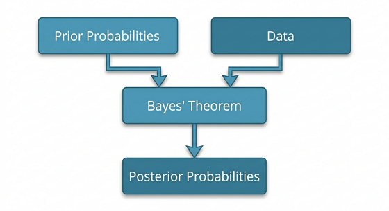
Fig. 1. The Bayesian Paradigm

The Bayesian paradigm differs from other statistical approaches in that, before the data D are obtained, the statistician evaluates the degrees of confidence in possible models and expresses them as probabilities. As soon as the data become available, Bayes' theorem allows us to recalculate these probabilities, taking the new information into account.

Thus, Bayesian methods are approaches to solving statistical problems in which Bayes' theorem serves as the tool for updating knowledge. Next, we will examine how it works in the discrete and continuous cases.

Bayes' Theorem: The Discrete Case

In the discrete case, we consider a finite list of hypotheses (also called models) H = {H1, H2, ..., Hk}. These hypotheses are mutually exclusive and, taken together, cover all possible explanations for the observed situation. Before receiving the data, we assign a prior probability to each hypothesis:

{P(H1), P(H2), ..., P(Hk)}

with two natural conditions satisfied:

• Each probability lies in the interval (0, 1),
• The sum of all prior probabilities is equal to 1.

Each model determines the probability of the observed data D occurring, assuming that this particular model is correct. These probabilities are expressed as conditional probabilities:

{P(D|H1), P(D|H2), ..., P(D|Hk)}

In the context of Bayesian inference, they are commonly referred to as likelihoods.

The revised probability values are denoted as:

{P(H1|D), P(H2|D), ..., P(Hk|D)}

Bayes' theorem (discrete case): Let {H1, H2, ..., Hk} be an exhaustive set of mutually exclusive statistical hypotheses, P(Hi) be the prior probabilities, P(D|Hi) be the likelihoods, and P(D) > 0. Then the posterior probabilities are given by the formula:

Here, P(D) is calculated using the law of total probability and serves as the normalizing constant.

Bayes' formula may seem complicated at first glance, but it actually follows directly from the definition of conditional probability. Let's recall the basic rule: the probability that both events H and D occur can be written in two ways:

• P(H ∩ D) = P(D | H) P(H)
• P(H ∩ D) = P(H | D) P(D)

Since the left-hand sides are equal, we can equate the right-hand sides as well:

P(H | D) P(D) = P(D | H) P(H)

This is how Bayes' famous formula is derived. As you can see, there is no magic involved here. All calculations are based on the basic operations of multiplying and adding probabilities.

Let's move on to some specific examples.

The Coin Example

Suppose there are two coins: a fair coin with a probability of 0.5 of landing on heads, and an unfair coin with a probability of 0.1 of landing on heads. We choose one of the coins at random, flip it, and get heads: D = {H}. The question is: What is the probability that the chosen coin is the fair coin?

First, let’s define the set of models {H1, H2}, where H1 represents the fair coin and H2 represents the unfair coin.

Since the selection of the coin is random, the prior probabilities of these models are equal:

• P(H1) = 0.5
• P(H2) = 0.5

The likelihoods (conditional probabilities) given the conditions of the problem are:

• P(H|H1) = 0.5
• P(H|H2) = 0.1

Using the total probability formula, let's calculate P(D):

• P(H) = P(H|H1) * P(H1) + P(H|H2) * P(H2) = 0.5 * 0.5 + 0.1 * 0.5 = 0.3

Now let's find the probability we are interested in using Bayes' formula:

• P(H1|H) = (0.5 * 0.5) / 0.3 = 0.833

Accordingly, for the second hypothesis:

• P(H2|H) = 1 - P(H1|H) = 0.167

Thus, before observing the data, our confidence that we had chosen the fair coin was 50%.

After the coin landed heads, it rose to 83%! The data significantly changed our initial probabilities.

An Infinite Set of Models

In the previous example, we worked with a finite list of hypotheses, but in the discrete case, an infinite set is also possible. In this case, all the results we have derived remain valid; only the number of hypotheses being tested changes.

Example: Bayesian analysis of the tick arrival rate for the EURUSD pair

Suppose that the number X of ticks received per minute for the EURUSD pair is a random variable with a Poisson distribution (Fig. 2). This model has one unknown parameter, θ — the average number of ticks per minute.

Since θ can take on any positive integer value (1, 2, 3, …), we obtain an infinite set of hypotheses {H₁, H₂, H₃, …}. Each of these hypotheses defines its own Poisson-type likelihood P(D|Hi), where Hi corresponds to the model θ = i.

Of course, in practice, we will still be limited to a certain finite subset of the most likely models. If we choose a sufficiently large number n, such that the combined probability of all hypotheses from H₁ to Hₙ is 99.99%, then the remaining 0.01% can be disregarded as statistically insignificant.

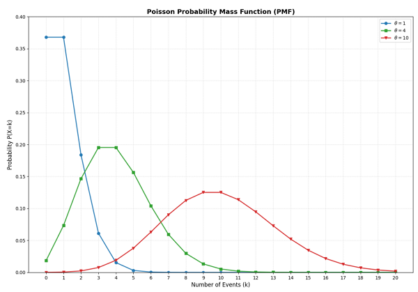
Fig. 2. Poisson Distribution

Suppose we have the following tick data for the last 10 minutes: D = [102, 82, 99, 132, 116, 122, 72, 78, 84, 92]. The arithmetic mean of this sample is 97.9. Let's assume that activity was higher last month — an average of 150 ticks. The Bayesian approach allows us to combine this experience with new data.

Formulation of an Informative Prior

As the prior distribution for the parameter θ, we will also use a Poisson distribution with a mean of 150 ticks. This reflects our prior knowledge that, on average, ticks arrive in the market at this rate. For the numerical calculation, we will use the grid approximation method. We will create an array of 300 hypotheses (θ ∈ [1, 300]), where each point represents a separate model with its own fixed mean value.

import pandas as pd
import numpy as np
import MetaTrader5 as mt5
from datetime import datetime
import pytz
from scipy.stats import poisson
from scipy.special import logsumexp
import matplotlib.pyplot as plt

# Initialize MT5 
if not mt5.initialize():
    print("initialize() failed")
    quit()

timezone = pytz.timezone("Etc/UTC")
target_date = (2026, 4, 23) 

utc_from = datetime(*target_date, 12, 0, 0, tzinfo=timezone)
utc_to = datetime(*target_date, 12, 10, 0, tzinfo=timezone)

# Load the ticks
ticks = mt5.copy_ticks_range("EURUSD", utc_from, utc_to, mt5.COPY_TICKS_ALL)
mt5.shutdown()

# Create a DataFrame and counting ticks per minute
df = pd.DataFrame(ticks)
df['time'] = pd.to_datetime(df['time'], unit='s')
df.set_index('time', inplace=True)
# Group by minute
minute_counts = df.resample('1min').count()['ask'].values

print(f"Data (number of ticks per minute): {minute_counts}")

sum_x = np.sum(minute_counts)
n = len(minute_counts)

# 1. Hypothesis grid
theta_grid = np.arange(1, 301)

# 2. Prior 
prior = poisson.pmf(theta_grid, mu=150)
prior /= prior.sum()

# 3. Likelihood
log_likelihood = sum_x * np.log(theta_grid) - n * theta_grid

# 4. Calculate the logarithm of the numerator (likelihood + prior)
log_numerator = log_likelihood + np.log(prior + 1e-12) # a vector with 300 elements

# 5. Find the logarithm of the total probability P(D) using LogSumExp
log_evidence = logsumexp(log_numerator)

# 6. Obtain the normalized log posterior
log_posterior = log_numerator - log_evidence

# 7. The final result on the probability scale
posterior = np.exp(log_posterior)

print(f"Sum of probabilities: {np.sum(posterior)}")
print(f"Log evidence: {log_evidence:.4f}")

# Likelihood normalization for visualization
log_evidence_likelihood = logsumexp(log_likelihood)
likelihood_norm = np.exp(log_likelihood - log_evidence_likelihood)

# --- Visualization ---
plt.figure(figsize=(10, 5))

# Prior 
plt.plot(theta_grid, prior, label='Prior',color='blue', linestyle='--', alpha=0.6)

# Likelihood 
plt.plot(theta_grid, likelihood_norm, label='Likelihood (Normalized Data)', 
         color='green', linewidth=1, alpha=0.8)

# Posterior 
plt.plot(theta_grid, posterior, label='Posterior', color='red', linewidth=2)

plt.fill_between(theta_grid, posterior, color='red', alpha=0.1)

# Maximum likelihood estimate (MLE)
plt.axvline(sum_x/n, color='green', linestyle=':', alpha=0.8,label=f'Data Mean: {sum_x/n:.2f}')

plt.title(f"Discrete Bayesian Inference (EURUSD)\nMinutes: {n}, Total Ticks: {sum_x}", fontsize=12)
plt.xlabel("Ticks per Minute (θ)")
plt.ylabel("Probability")
plt.legend()
plt.grid(True, alpha=0.2)
plt.show()

print(f"Sample mean (MLE): {sum_x/n:.2f}")
print(f"Most probable value (MAP): {theta_grid[np.argmax(posterior)]}")

Since the Poisson series is theoretically infinite but our model grid is bounded, we normalize the prior weights so that their sum is exactly 1.

prior = poisson.pmf(theta_grid, mu=150)
prior /= prior.sum()

Now each hypothesis has its own prior probability.

Working with likelihood

The Poisson model for a single observation with a given mean θ is calculated as follows:

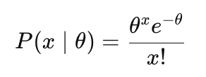
However, since we have an entire dataset D rather than a single number, and we assume that tick counts in different minutes are independent, the overall likelihood is the product of the probabilities for each data point:

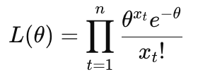
Working with products of powers and exponentials is inconvenient (the numbers become too small for a computer to represent). Therefore, we take the natural logarithm of the likelihood, ln(L). Taking the logarithm turns a product into a sum and brings an exponent down as a factor:

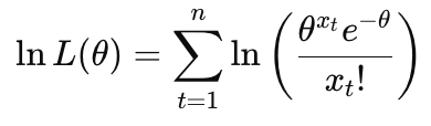
Let's break down the logarithm of the fraction into its components:

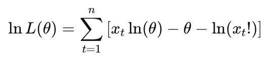
When performing the calculation on a computer, we compute only the first and second terms of the sum, since the logarithm of the factorial is a constant that does not depend on the parameter θ.

# 3. Likelihood
log_likelihood = sum_x * np.log(theta_grid) - n * theta_grid

In Bayesian inference, the only parts of the formula that matter to us are those that contain our unknown parameter θ. Therefore, there is no need to calculate the logarithm of the factorial.

The posterior and the law of total probability

Now we will combine all the components into a single system. To obtain the posterior, we need to multiply the prior by the likelihood. Since we are working in logarithmic space, multiplication becomes addition:

log_numerator = log_likelihood + np.log(prior + 1e-12) 

Here, log_numerator is a vector with 300 elements. Each value in the vector corresponds to one of our 300 models. Currently, the sum of the (unnormalized) weights obtained for the 300 models is not equal to 1. To obtain the probabilities, we need to calculate the normalization constant P(D) and divide the values by it. In Bayesian statistics, the total probability of the data, P(D), is also referred to as "evidence" or marginal likelihood. Mathematically, P(D) is the sum of the products of the likelihood and the prior across all 300 of our models. In other words, it is the expected value of the likelihood with respect to the prior distribution.

To ensure numerical stability when calculating P(D), we will use the logsumexp function. It computes the logarithm of a sum of exponentials while avoiding memory overflow when working with very large or very small numbers:

log_evidence = logsumexp(log_numerator)

Fig. 3 shows the results of the calculations.

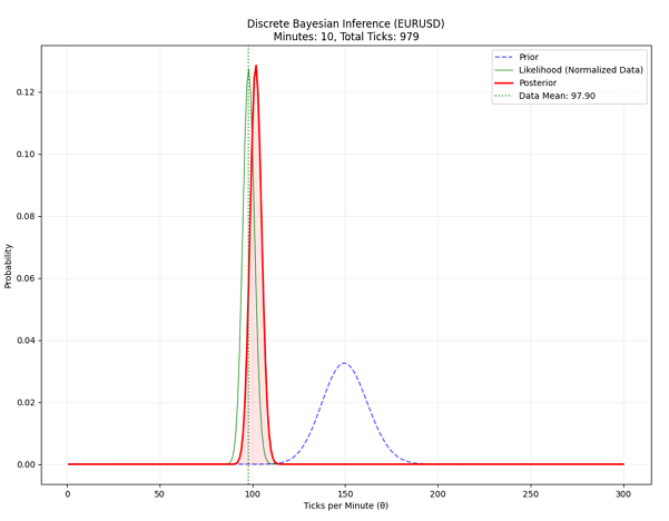
Fig. 3. Bayesian inference for the Poisson model

We can see how the initial prior (our expectation of 150 ticks) has shifted and changed shape under the influence of new data, forming an up-to-date representation of the current tick arrival rate.

It is important to note that the prior and posterior are probability distributions: the probabilities in each always sum to 1.0. Likelihood is on a different scale and can take on any value. To plot the likelihood on the same graph as the prior and posterior, it must be brought to the same scale (normalized). To do this, we:

• calculate the total “mass” of the likelihood using `logsumexp(log_likelihood)`,
• divide each log-likelihood value by this total mass (in log space, this is simply subtraction).

Bayes' Theorem: The Continuous Case

Up to this point, we have been working with discrete hypotheses: the coin is either fair or not; the mean number of ticks is any integer from 1 to 300, and so on. However, in most practical situations, we have to deal with an uncountable (continuous) set of possible values for the parameter.

Let's consider a binomial distribution model, where we are interested in the probability of success, θ. Here, the parameter θ can take any value in the unit interval [0, 1]. It is no longer possible to compile a complete list of hypotheses and assign a probability to each one — there are an infinite number of them.

Instead, we describe our degree of belief in different values of the parameter θ using a probability density function — a continuous curve. Where the curve is higher, our prior expectations are stronger. Where it is close to zero, we consider such values of θ to be unlikely.

Thus, a discrete prior in the form of a table or grid of values becomes a smooth curve, and the mathematics shifts from simple summation to integration (calculating the area under this curve).

Bayes' theorem (continuous case): Let Θ be the parameter space, θ ∈ Θ, p(θ) the prior density, and p(D|θ) the likelihood. Then the posterior density p(θ|D) is given by:

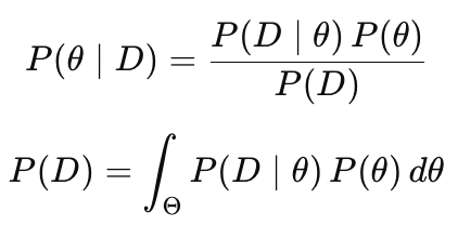
• P(D) — Evidence (Marginal Likelihood): In the continuous case, this is an integral over the entire space of possible values of the parameter θ.

When moving to continuous models, the problem becomes considerably more complex mathematically. While normalization in the discrete case simply involved adding a few numbers, we now need to compute an integral.

In our example with a single parameter θ, this still seems manageable. But as soon as we move on to real-world machine learning problems, where there may be tens, hundreds, or thousands of parameters, we run into the curse of dimensionality. A multidimensional integral over a vast parameter space is often impossible to compute analytically.

It is precisely because of this computational complexity that Bayesian statistics remained in the shadow of classical methods for a long time. It was only with the advent of powerful computers and specialized algorithms (such as Markov chain Monte Carlo methods — MCMC) that the Bayesian approach became a truly practical tool.

There is another way to make a researcher's life easier — by using what are known as conjugate distributions. They allow you to obtain an exact result using simple arithmetic operations, avoiding cumbersome integrals altogether. This is the path we will take next.

Choosing a Prior Distribution in the Continuous Case

It should be noted that there is no single correct prior for every situation. This choice depends on the specific task and the researcher's experience. Here, just as in trading, there is some room for creativity.

Consider Fig. 4, which shows various types of prior densities P(θ) for a binomial distribution with an unknown parameter θ.

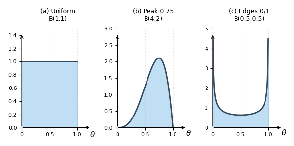
Fig. 4. Possible prior distributions P(θ) for the binomial distribution

• In case (a), we assume that all values of the parameter θ in the range 0 ≤ θ ≤ 1 are equally likely. In this situation, the model has no initial preferences and will rely entirely on the data,
• In case (b), we assume that the most likely value of the parameter is θ = 0.75,
• In case (c), we assume that values of θ close to 0 and 1 are more likely than values in the center.

There may be a sense that the choice of one type of prior distribution over another is somewhat subjective. Indeed, two statisticians may choose different prior distributions for the same problem.

Instead of relying on intuition, we can use empirical analysis:

• collect historical data for past periods,
• construct a histogram of the distribution of the parameter of interest,
• fit a suitable mathematical model (a beta distribution, a gamma distribution, etc.) to this histogram.

Thus, your prior ceases to be merely an opinion and becomes a condensed summary of past observations.

Bayesian inference in the beta-binomial model

Recall that the binomial model describes the probability of obtaining y successes (data D) in n independent trials, given a fixed probability of success θ.

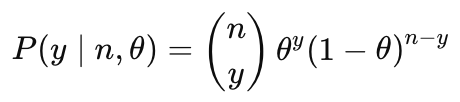
Theoretically, we could compute the posterior distribution for this model numerically (on a grid), just as we did in the Poisson example. However, when working with continuous parameters, this approach becomes too cumbersome.

Fortunately, Bayesian statistics offers conjugate distributions (conjugate priors). These are special pairs of distributions that are mathematically a perfect match for one another: when the prior is multiplied by the likelihood, the result retains the same functional form as the original prior. For the binomial likelihood, the conjugate prior is the beta distribution. We have already seen several examples of such curves in Fig. 4. The main advantage of conjugate distributions is that they allow us to completely avoid complex integrals. The solution is obtained in closed form (analytically).

If the prior is specified as Beta(a, b), and our observations yield y successes and (n−y) failures, then the posterior parameters are calculated very simply:

Beta (θ|a + y, b + n - y)

Thus, the posterior distribution once again takes the form of a beta distribution, but with updated parameters.

Let's see how the prior beliefs shown in Fig. 4 are updated if we conduct 10 trials in which we obtain 8 successes (y) and 2 failures (n-y). The graphs below (Fig. 5) show the corresponding posterior distributions.

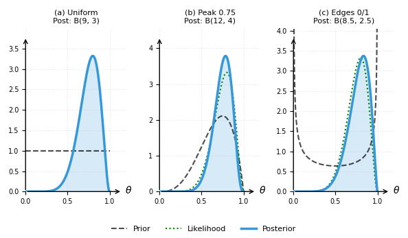
Fig. 5. Posterior distributions P(θ|D) for the binomial likelihood

Final result:

• Case (a): The posterior distribution became Beta(1+8, 1+2) = Beta(9, 3). The curve fully reflects the data: the maximum is around 0.8,
• In case (b), the posterior became even narrower, indicating greater certainty, since the data confirmed the prior expectation,
• In case (c), the data completely overwhelmed the initial belief in the extremes (0 or 1), causing the curve to become concentrated closer to the center. Although the posterior distribution here is slightly broader than in case (a), it clearly demonstrates that a sufficient amount of data can correct even the most exotic prior distribution.

Posterior mode: MAP estimate

Ultimately, we often need a single specific value for the parameter θ. For this, we can use the maximum a posteriori (MAP) estimate. In other words, we are looking for the mode of the posterior distribution — the point where the probability density is maximized:

For the beta-binomial model, this value is calculated using a very simple analytical formula:

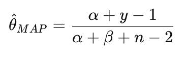
In the case of a uniform prior, the MAP estimate reduces to the maximum likelihood estimate (MLE). For example, if we substitute the values for the uniform prior into the formula, we get (1 + 8 - 1) / (1 + 1 + 10 - 2) = 8/10. This estimate is intuitive, but it can be very far from the truth if the data sample is small.

For example, we flipped a coin 5 times, and it landed on heads all 5 times. In that case, the maximum likelihood estimate of the probability of tails is 0, meaning it predicts that tails will never occur in the future. Naturally, this is a poor estimate because it is based on insufficient data.

If we add a prior (for example, Beta(2,2)), our knowledge will be updated to Beta(2+5, 2+0) = Beta(7, 2). The MAP estimate will be (7−1) / (7+2−2) = 6/7 ≈ 0.85. Thus, the Bayesian model acknowledges that there is a bias toward heads, but it still assigns a nonzero probability to tails.

Posterior mean

The posterior mode (MAP) shows us the most likely value of the parameter. However, it may provide an incomplete or even distorted picture because it completely ignores the shape of the distribution around that peak — how broad it is, whether it is symmetric, or whether it has heavy tails.

The posterior mean, on the other hand, is a more robust estimate. It takes into account the entire distribution and is obtained by averaging (integrating) over all possible values of θ, weighted by their probabilities.

This estimate is a combination of the prior mean and the MLE. The weaker the prior distribution, the closer the posterior mean is to the MLE.

For our example with 8 successes and 2 failures, the posterior mean is:

E[θ|D] = (1 + 8) / (1 + 1 + 10) = 0.75

Posterior Predictive Distribution

Estimating the parameters (θ) is only an intermediate step. The true purpose of Bayesian analysis is to make predictions about new, as-yet-unobserved data. In the Bayesian approach, this problem is solved using the posterior predictive distribution.

To answer the question, “What is the probability of success (ynew) in the next trial?”, we do not choose a single “best” value for θ. Instead, we conduct a weighted vote among all possible models. Each model provides its own forecast, and we assign a weight to it that is proportional to how much we believe in it after the update (that is, according to the posterior distribution). Mathematically, this means that we need to integrate the likelihood with respect to the posterior distribution of θ.

Fortunately, for the beta-binomial model, this complex process of weighted voting for a single subsequent trial (n = 1) is greatly simplified and reduces to a simple ratio:

You have probably noticed that the prediction formula is exactly the same as the formula for the posterior mean. This perfect match is a distinctive feature of the beta-binomial model. In more complex models, the posterior mean and the predictive distribution generally differ.

Dynamic Bayesian Updating

In many practical situations, data arrive sequentially over time {D₁, D₂, ..., Dt}, as in a stream of quotes. Under these circumstances, we do not wait for the entire sample to be collected. Instead, we update our beliefs immediately after receiving each new observation: first, we analyze the data D₁, then we revise our probabilities as D₂ arrives, and so on. This process is called dynamic Bayesian updating (illustrated schematically in Fig. 6).

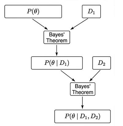
Fig. 6. Dynamic Bayesian updating

Or, expressed as a formula:

where

• P(θ∣D1:t) — the new posterior (after step t),
• P(Dt|θ) — the likelihood of the current observation,
• P(θ|D1:t-1) — the prior, which is actually the posterior from the previous step.

Let's consider a simple example of dynamic Bayesian updating:

import numpy as np
import matplotlib.pyplot as plt

# 1. Simulate sequential data arrival
data = [1, 1, 0, 1, 1, 1, 0, 1, 1, 1] # 1 - increase, 0 - decrease

# 2. Initial prior parameters (Uniform Prior)
alpha_current = 1
beta_current = 1

history = []

print(f"{'Step':<5} | {'Data':<7} | {'Alpha':<6} | {'Beta':<5} | {'MAP':<6} | {'Mean (Forecast)':<10}")
print("-" * 60)

# 3. Sequential updating loop (Bayesian Updating)
for i, y in enumerate(data):
    
    # UPDATE: add a success or failure
    if y == 1:
        alpha_current += 1
    else:
        beta_current += 1
        
    # MAP (mode)
    if alpha_current + beta_current > 2:
        map_val = (alpha_current - 1) / (alpha_current + beta_current - 2)
    else:
        map_val = 0.5 # For a uniform distribution, the mode is not uniquely defined 
        
    mean_val = alpha_current / (alpha_current + beta_current)
    
    history.append((alpha_current, beta_current, mean_val))
    
    print(f"{i+1:<5} | {y:<7} | {alpha_current:<6} | {beta_current:<5} | {map_val:<6.3f} | {mean_val:<10.3f}")

# 4. Visualize the learning process
steps = np.arange(1, len(data) + 1)
means = [h[2] for h in history]

plt.figure(figsize=(8, 4), dpi=100)
plt.step(steps, means, where='post', color='#3498db', lw=2, label='Posterior Mean (Forecast)')
plt.axhline(0.5, color='gray', linestyle='--', alpha=0.5, label='Initial Prior (0.5)')

plt.title('Step-by-step Bayesian Updating', fontsize=12)
plt.xlabel('Observation Number (Time)', fontsize=10)
plt.ylabel('Probability of Success', fontsize=10)
plt.ylim(0, 1)
plt.grid(True, linestyle=':', alpha=0.6)
plt.legend()
plt.show()

Figure 7 shows how the forecast evolves through sequential updating as the number of observations increases.

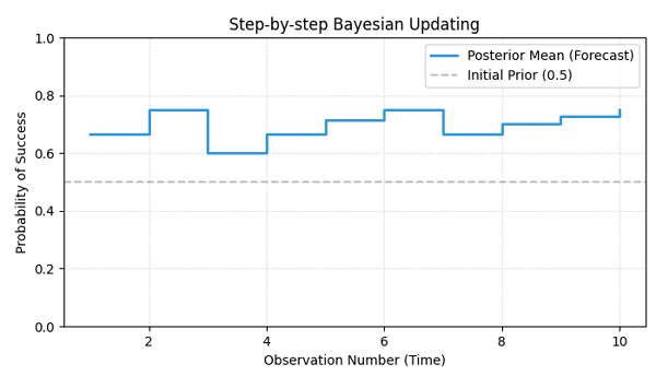
Fig. 7. Forecast Based on the Posterior Mean

Let's discuss the nuances of applying this approach to nonstationary financial data. All of our previous calculations were based on the implicit assumption that the rules of the game would remain unchanged. In statistics, this is called stationarity. When studying stationary processes, the more data we have, the more accurately we can estimate their parameters.

In the nonstationary case, this is not true. The market regime (the data-generating process) can change at any time. In such a situation, old data not only ceases to be helpful but actually begins to cause harm: the model continues to rely on rules that no longer work.

It stands to reason that more recent data should carry more weight than observations from a week or a month ago. To implement this idea, we introduce a forgetting factor, gamma (γ), into the model. We will modify the previous code by adding this parameter. Essentially, γ controls how quickly the model forgets old data:

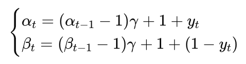
• If γ = 1, the model remembers the entire history and performs standard Bayesian updating,
• If γ < 1, the model gradually forgets the past and responds more strongly to recent observations.

The relationship between this forgetting factor and the familiar moving window is expressed by a simple formula:

n = 1/(1 - γ)

For example, if we want the model to make decisions based on the last 20 candlesticks, we set γ = 0.95.

Example: A simple change-point detection indicator

To demonstrate how the algorithm works, synthetic data was generated to simulate a sudden change in the market regime. In the first half of the sequence (the first 100 observations), the probability of success was θ = 0.6 (an upward trend). In the second half, the parameter changed sharply to θ = 0.3 (a downward trend).

import pandas as pd
import numpy as np
import matplotlib.pyplot as plt

# 1. Generate synthetic data
# First, an upward trend (60% probability of an upward move), then a sharp downward reversal (30% probability of an upward move)
np.random.seed(42)
data_up = np.random.choice([1, 0], size=100, p=[0.6, 0.4])
data_down = np.random.choice([1, 0], size=100, p=[0.3, 0.7])
data = np.concatenate([data_up, data_down])

# 2. Model parameters
gamma = 0.94  # Forgetting factor gamma (the smaller γ is, the faster the model forgets the past)
a_curr, b_curr = 1, 1 # Initial parameters: Beta(1,1) — uniform prior

history = []

# 3. Dynamic Bayesian updating loop with exponential decay
for y in data:
    #  Add 1 to ensure that we always retain at least a baseline Beta(1,1) prior
    a_curr = (a_curr - 1) * gamma + 1
    b_curr = (b_curr - 1) * gamma + 1
    
    # Update with a new observation
    if y == 1:
        a_curr += 1
    else:
        b_curr += 1
        
    # Calculate the current posterior mean (expected probability of success)    
    mean = a_curr / (a_curr + b_curr)
    history.append(mean)

# 4. Visualization
plt.figure(figsize=(12, 5), dpi=100)
plt.plot(history, color='#3498db', lw=2, label=f'Adaptive Bayesian (gamma={gamma})')
plt.axhline(0.5, color='black', linestyle='--', alpha=0.3)
plt.axvline(100, color='red', linestyle=':', label='Change point')

# 5. Compare with standard (non-adaptive) Bayesian updating (gamma=1)
a_std, b_std = 1, 1  # We'll also start with a uniform prior, Beta(1,1)
std_history = []
for y in data:
    # Standard Bayesian updating — we simply add each new observation
    if y == 1: a_std += 1
    else: b_std += 1
    mean_std = a_std / (a_std + b_std) # Posterior mean
    std_history.append(mean_std)

plt.plot(std_history, color='gray', alpha=0.5, label='Standard Bayesian (gamma=1.0)')

plt.title('Adaptive Bayesian Update vs Standard', fontsize=12)
plt.legend()
plt.grid(alpha=0.2)
plt.show()

As shown in Fig. 8: standard Bayesian updating responds to a regime change with a noticeable delay.

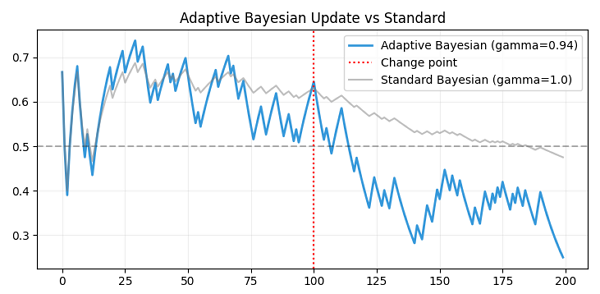
Fig. 8. Comparison of forecasts using adaptive and standard Bayesian updating

In contrast, the adaptive version with a forgetting factor of γ = 0.94 responded significantly faster — it required approximately 17–20 new observations to reliably detect a change in the market. This period agrees very well with the moving window size calculated using the formula n = 1/(1 − 0.94) ≈ 16.7.

Thus, we have obtained a simple yet effective change point detection indicator based on a Bayesian beta-binomial model with exponential decay.

To reproduce the results shown here, you will need a Python interpreter and the standard set of statistical packages. For instructions on how to install them, see the article “Python + MetaTrader 5: A Quick Research Loop for Data, Features, and Prototypes.”

After installing the packages, place the files attached to this article in a single folder (for example, Scripts/BayesianInference).

To view the graphs, run the script using MetaEditor:

• In MetaEditor, click File → Open and select the desired .py file from the BayesianInference folder,
• After opening the file, press the F7 key (or click the "Compile" button on the toolbar),
• The graph should appear in a separate window.

Conclusion

In this article, we have followed the full path from the philosophical foundations of the Bayesian paradigm to practical data analysis tools. Using the examples of discrete and continuous models, we have seen how prior experience and actual data are transformed into updated knowledge — the posterior distribution.

The Bayesian approach is characterized by intellectual honesty in the face of uncertainty: it explicitly balances accumulated historical knowledge and new data, avoiding the false confidence often exhibited by classical frequentist methods with small samples.

Using the beta-binomial model as an example, we were introduced to the concept of conjugate distributions. These distributions reduce Bayesian inference to simple arithmetic operations, making the algorithm fast and suitable for real-time data analysis.

Special attention was given to the sequential Bayesian updating mechanism, which allows the model to dynamically revise its beliefs as new information becomes available.

We hope that understanding the basic principles of Bayesian inference will help you in your further study of probabilistic machine learning and in your practical work with uncertainty.

Software used in this article

#	Name	Type	Description
1	Poisson.py	Script	Bayesian inference for the tick arrival rate using the Poisson model
2	BayesianUpdating.py	Script	Sequential updating of the forecast in the beta-binomial model
3	AdaptiveUpdate	Script	Adaptive sequential updating of the forecast in the beta-binomial model