

A Categorical Hidden Markov Model in MQL5
 78
 2

Introduction
State space models (SSM) are a fundamental mathematical framework for analyzing and forecasting sequential data. They are widely used in signal processing, genetics, econometrics, and other fields.
At the heart of any state-space model lies the joint probability distribution of the observed sequence y1, …, yT. A key assumption of the SSM is that the observed process is generated by a sequence of hidden (latent) states z1, …, zT, whose evolution over time is described by a transition model.
Depending on the nature of the latent states (discrete or continuous), the type of transition dynamics (linear or nonlinear), and the type of observations (categorical, Gaussian, or Poisson), SSMs are divided into different classes.
The subject of this article is the categorical hidden Markov model (HMM) — a classic example of the SSM class with discrete latent states and a categorical distribution of observed data. Transitions between states in the system are described using a transition probability matrix.
For example, the model allows you to identify hidden market regimes based on a sequence of market events (white or black candles). In one regime (let's call it an uptrend), white candles appear much more frequently; in another (a downtrend), black candles are more common; and in a third (a sideways market), their probabilities are equal. Of course, we do not observe the regimes themselves; they are hidden. The model's goal is to infer the current market state by analyzing only the available data (candlestick colors).
To test such hypotheses, the CCategoricalHMM class was implemented in MQL5. Using simple and clear examples, we will explore the class's main features:- calculation of posterior probabilities of hidden states (Inference),
- learning the model parameters using the EM algorithm (Fit),
- synthetic data generation (Sample),
- selecting the optimal number of latent states using the AIC and BIC criteria (Model Selection),
- real-time online filtering of hidden states (Filter).
Categorical Hidden Markov Model
It is common practice to represent the structure of a hidden Markov model graphically as a directed acyclic graph.
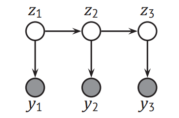
Fig. 1. An HMM represented as a graph
In the diagram shown (Fig. 1), the elements of the graph have the following meanings:
- nodes (circles) — random variables,
- white nodes (zt) — hidden variables that cannot be directly observed,
- dark nodes (yt) — observed variables,
- directed edges (arrows) — probabilistic dependencies between variables.
The graph shows that each hidden state zt depends only on the previous state zt−1. This means that the sequence of hidden states forms a first-order Markov chain. Furthermore, the observed variable yt depends solely on the current hidden state zt and is conditionally independent of all previous observations and states, given zt. This is an important assumption of the model — the conditional independence of the observations. Formally, this means the following: if the current regime of the system (zt) is known, then the preceding observation history and past hidden states provide no additional information for predicting the current observation.
The structure described here is a standard HMM. However, there are also extensions of this model — for example, autoregressive hidden Markov models (AR-HMM). These models add direct links between the observations themselves (yt-1 → yt), allowing them to account for short-term autocorrelation in the data.
The CCategoricalHMM class
Below is the class declaration and a brief description of its main components.
//+------------------------------------------------------------------+
//|                                               CategoricalHMM.mqh |
//|                                                           Eugene |
//|                                             https://www.mql5.com |
//+------------------------------------------------------------------+
#property copyright "Eugene"
#property link      "https://www.mql5.com"
#include <Math\Stat\Uniform.mqh>
#include <Math\Stat\Gamma.mqh>

//+------------------------------------------------------------------+
//|Categorical Hidden Markov Model                                   |
//|Categorical Hidden Markov Model                                   |
//+------------------------------------------------------------------+
class CCategoricalHMM
  {
public:
   // --- Main model parameters ---
   int               m_numStates;      // Number of hidden states
   int               m_numEmissions;   // Number of possible observable symbols
   matrix            m_TR;             // Transition Matrix (m_numStates × m_numStates)
   matrix            m_E;              // Emission Matrix    (m_numStates × m_numEmissions)

   //--- Priors (regularization) ---
   matrix            m_pTR;            // Prior pseudocounts for transitions
   matrix            m_pE;             // Prior pseudocounts for emissions

   vector            m_logliks;        // Log-likelihood history
private:
   int               m_seed;           // Seed for reproducible generation of pseudorandom numbers
public:

   // --- Constructors ---
                     CCategoricalHMM(int numStates, int numEmissions, int seed = -1);
                     CCategoricalHMM(int numStates, int numEmissions,
                   const matrix &pTR, const matrix &pE, int seed = -1);

   // --- Main methods ---
   bool              Fit(const vector &y, int maxIter = 100, double tolerance = 1e-6,
                         bool verbose = false); // Baum-Welch training

   bool              Inference(const vector &y, const matrix &tr, const matrix &e,
                               matrix &Sdist, double &LL, matrix &Fdist, matrix &bs, vector &s); // Forward-Backward

   bool              Sample(int T, const matrix &tr, const matrix &e, vector &y, vector &z); // Sample generation

   // --- Online filtering ---
   vector            Filter(const vector &PrevState, int nextObs);

   // --- Information criteria ---
   double            AIC(double logLike) {return -2.0 * logLike + 2.0 * GetParams();}
   double            BIC(double logLike, int n_samples) {return -2.0 * logLike + GetParams() * MathLog(n_samples);}
   int               GetParams(); // Number of model parameters

   // --- Initialize parameter matrices with random values ---
   bool              RandomDirichlet(const double &alpha[], double &result[]);
private:
   matrix            RandomizeMatrix(int rows, int cols, const double &alpha[]);
  };
Main methods of the class:
- Fit() — model training. Implements the classic Baum-Welch EM algorithm. Given a sequence of observations, it finds the optimal transition matrix (m_TR) and emission matrix (m_E) by maximizing the log-likelihood,
- Inference() — posterior inference. Implements a scaled forward-backward algorithm. Calculates the marginal log-likelihood (LL), as well as the filtering (Fdist), smoothing (Sdist), and backward probability matrices required for training and forecasting,
- Sample() — synthetic data generation. A Monte Carlo method that generates sequences of hidden states and their corresponding observations from the specified TR and E matrices,
- Filter() — online filtering. A recursive Bayesian filter for real-time operation. Based on the previous state distribution and the new observation, it updates the probabilities of the current hidden states.
The HMM training process is sensitive to initial conditions and may encounter the problem of zero probabilities. With classical maximum likelihood estimation (MLE) on limited samples, zero entries can easily arise in the matrices if a particular symbol or transition did not occur in the training data.
To address this issue, the class implements Bayesian regularization using prior pseudocounts (m_pTR and m_pE). Pseudocounts smooth the estimates and prevent state degeneracy. Even if a particular pattern has never occurred in the past, it retains a small, nonzero probability of occurring in the future.
The helper methods RandomDirichlet() and RandomizeMatrix() are used to initialize matrices randomly. The Dirichlet distribution allows us to generate matrix rows in which the sum of the elements is exactly 1, ensuring valid probability distributions from the very beginning of training.
In addition, the class implements methods for calculating the AIC and BIC information criteria. They allow us to estimate the optimal number of hidden states, striking a balance between the model's fit and its complexity.
An Experiment with Dice
To clearly illustrate how the categorical model works, let's consider an experiment with dice.
Let's say we have two dice with numbers from 1 to 6 on their faces. The first is a fair die (Fair), for which the probability of rolling each face is 1/6. The second is a loaded die (Loaded), biased toward rolling a six.
At each step, one of the dice is selected according to certain rules (Fig. 2) and rolled, and the result is recorded; the same die may then be kept or replaced. The problem is as follows: given only the sequence of numbers rolled (observations), determine which specific die was used in each roll.
Let's translate the conditions of the experiment into the language of state-space models:
- The latent variable (z) takes on two discrete values, z ∈ {1, 2}, where 1 represents a fair die (Fair) and 2 represents a loaded die (Loaded),
- The observed variable (y) takes on six discrete values, y ∈ {1, 2, 3, 4, 5, 6}, corresponding to the faces rolled.
The dynamics of switching between dice are described by the state transition matrix (TR). In Fig. 2, the arrows indicate the transition probabilities, where the probability of remaining in the first state is 0.95 and the probability of transitioning to the second state is 0.05. Similarly, if we are currently in the second state, the probability of remaining in that state is 0.9, and the probability of returning to the first state is 0.1.
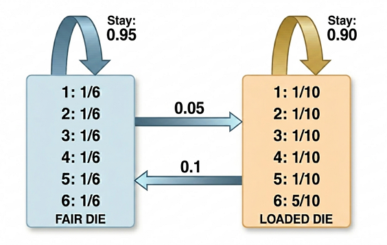
Fig. 2. Transition matrix TR and emission matrix E
The second key component of the model is the emission matrix (E). It specifies the categorical probability distribution over the die faces for each hidden state:
- For the fair die (Fair): the distribution is uniform — the probability of rolling any of the six faces is 1/6,
- For the loaded die (Loaded): the probability of rolling a six is 0.5, while the probability of rolling each of the other five faces is 0.1.
The process of inferring hidden states for this example is demonstrated in the Inference.mql5 script.
Hidden State Inference (Inference)
//+------------------------------------------------------------------+
//|                                                    Inference.mq5 |
//|                                                           Eugene |
//|                                             https://www.mql5.com |
//+------------------------------------------------------------------+
#property copyright "Eugene"
#property link      "https://www.mql5.com"
#property version   "1.00"
#include <CategoricalHMM\CategoricalHMM.mqh>
#include <Graphics\Graphic.mqh>
//+------------------------------------------------------------------+
//| Script program start function                                    |
//+------------------------------------------------------------------+
void OnStart()
  {
   int n_states = 2;    // Number of hidden states
   int n_emissions = 6; // Number of possible outcomes (number of classes)

// --- 1. Create a model (seed=99 for reproducibility) ---
   CCategoricalHMM model(n_states, n_emissions, 99);

// --- Set the model parameters ---
// --- 2. Transition matrix TR ---
   matrix tr = {{0.95, 0.05},
        {0.1,  0.9}
     };
// --- 3. Emission matrix (E) ---
   matrix e = {{1.0/6, 1.0/6, 1.0/6, 1.0/6, 1.0/6, 1.0/6},
        {0.1,   0.1,   0.1,   0.1,   0.1,   0.5}
     };

// --- 4. Generate a sequence of observations and hidden states ---
   vector y;
   vector z;
   int n_samples = 300; // Number of samples to generate
   model.Sample(n_samples, tr, e, y, z);

   PrintFirst(z,"First 5 states",5);       // First 5 states:     [1 1 1 1 1]
   PrintFirst(y,"First 5 emissions",5);    // First 5 emissions:  [6 1 5 2 3]

// --- VISUALIZATION SECTION ---
   int plotLimit = 300; // Plot the first 300 points
   double x[], y_[];
   ArrayResize(x, plotLimit);
   ArrayResize(y_, plotLimit);
   for(int i = 0; i < plotLimit; i++)
     {
      x[i] = i;
      y_[i] = z[i];
     }
   ChartSetInteger(0,CHART_SHOW,false);
   CGraphic graphic;
   ulong width = ChartGetInteger(0,CHART_WIDTH_IN_PIXELS);
   ulong height = ChartGetInteger(0,CHART_HEIGHT_IN_PIXELS);
   graphic.Create(0,"HMM_States_Plot",0,0,0,int(width),int(height));
   CCurve *curve = graphic.CurveAdd(x, y_, ColorToARGB(clrDodgerBlue, 255), CURVE_LINES,"States");
   curve.LinesStyle(STYLE_SOLID);
   curve.LinesWidth(2);
   graphic.BackgroundMainColor(ColorToARGB(clrBlack,255));
   graphic.BackgroundMainSize(24);
   graphic.BackgroundMain("States over time");
   graphic.XAxis().Name("Time");
   graphic.XAxis().NameSize(18);
   graphic.YAxis().Name("State (1=Fair, 2=Loaded)");
   graphic.YAxis().NameSize(18);
   graphic.YAxis().Min(1);
   graphic.YAxis().Max(2);
   graphic.CurvePlotAll();
   graphic.Update();
   Sleep(5*1000);
   ChartSetInteger(0,CHART_SHOW,true);
   graphic.Destroy();
   ChartRedraw(0);

// --- Empirical probability of observing a 6 for the fair die (Fair) and the loaded die (Loaded) ---
   PrintFormat("Empirical probability '6' (Fair): %.3f", CalculateSixFreq(y, z, 1));
   PrintFormat("Empirical probability '6' (Loaded): %.3f", CalculateSixFreq(y, z, 2));

// --- Inference ---
   matrix Filtering, Smoothing, bs;
   double marginal_loglik;
   vector s;

   if(model.Inference(y,tr,e,Smoothing,marginal_loglik,Filtering,bs,s))
     {
      Print("---Inference---");
      PrintFormat("Log-likelihood (marginal_loglik): %.10f", marginal_loglik);
      Print("\nSmoothing matrix  (posterior probabilities):");
      PrintMatrixFormatted(Smoothing);
      Print("\nFiltering matrix :");
      PrintMatrixFormatted(Filtering);
     }
//MatrixToCSV("FilteringDist.csv", Filtering);
//MatrixToCSV("SmoothingDist.csv", Smoothing);
//VectorToCSV("TrueStates.csv", z);

  }
//+------------------------------------------------------------------+

//+-------------------------------------------------------------------+
//|Return the relative frequency of rolling a six                     |
//+-------------------------------------------------------------------+
double CalculateSixFreq(const vector &r, const vector &s, int stateTarget)
  {
   int count = 0, total = 0;
   for(int i=0; i<(int)r.Size(); i++)
     {
      if(s[i] == stateTarget)
        {
         total++;
         if(r[i] == 6)
            count++;
        }
     }
   return (total > 0) ? (double)count/total : 0;
  }
//+------------------------------------------------------------------+
We create an instance of the class, passing the following parameters to its constructor: numStates = 2 (the number of hidden states) and numEmissions = 6 (the number of possible outcomes). To ensure reproducibility of the results, the pseudorandom number generator seed is fixed (seed = 99). Next, the true model parameters — the transition and emission matrices — are specified. In this example, we assume that the model parameters are known to us in advance.
Let's sample 300 observations and hidden states from this model using the Sample method. The method takes as input the desired number of observations and the parameter matrices. The result is two synchronized vectors:
- the vector of true hidden states z (which die was rolled),
- the vector of observed outcomes y (which number came up).
Figure 3 shows the resulting sequence of states.
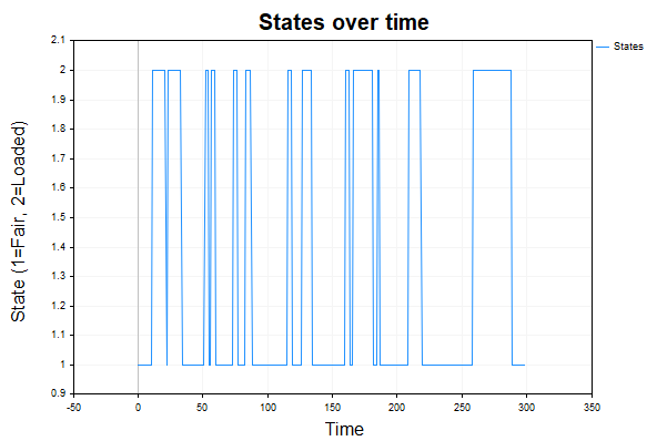
Fig. 3. Sequence of Hidden States
Before moving on to inferring hidden states, let's check the quality of the generated sample. To do this, we will calculate the empirical probabilities of rolling a six in each of the hidden states:
- Empirical probability '6' (Fair): 0.173,
- Empirical probability '6' (Loaded): 0.468
As can be seen, even with a relatively small sample of 300 observations, the empirical frequencies are quite close to the theoretical values (0.167 and 0.5, respectively). This confirms that the Sample() method is working correctly.
//+------------------------------------------------------------------+
//| Generation of a sequence of states and observations              |
//| based on the specified transition and emission matrices.         |
//|--------------- IN -----------------------------------------------|
//| int T           - length of the generated sequence               |
//| matrix &tr      - transition probability matrix                  |
//| matrix &e       - emission probability matrix                    |
//|--------------- OUT ----------------------------------------------|
//| vector &y       - generated sequence of observations             |
//| vector &z       - generated sequence of states                   |
//+------------------------------------------------------------------+
bool CCategoricalHMM::Sample(int T, const matrix &tr, const matrix &e,
                             vector &y, vector &z)
  {
   if(T <= 0)
      return false;

   int numStates = (int)tr.Rows();
   int numEmissions = (int)e.Cols();
   y.Resize(T);
   z.Resize(T);

//+------------------------------------------------------------------+
//|1. Preparing cumulative distribution functions (CDFs)             |
//|This allows for quick sampling from a categorical distribution    |
//+------------------------------------------------------------------+
   matrix trc = tr.CumSum(1);   // Row-wise cumulative sum (transitions)
   matrix ec  = e.CumSum(1);    // Row-wise cumulative sum (emissions)

//--- Normalization of cumulative sums (mapped to the range [0, 1]) ---
   vector tr_last_col = trc.Col(numStates - 1);
   vector e_last_col = ec.Col(numEmissions - 1);

   for(int r = 0; r < numStates; r++)
     {
      trc.Row(trc.Row(r) / tr_last_col[r], r);
      ec.Row(ec.Row(r) / e_last_col[r], r);
     }

//+------------------------------------------------------------------+
//|2. Random number generation                                       |
//+------------------------------------------------------------------+
   double statechange[];
   double randvals[];
   MathRandomUniform(0.0, 1.0, T, statechange);
   MathRandomUniform(0.0, 1.0, T, randvals);

//+------------------------------------------------------------------+
//|3. Sequence generation                                            |
//+------------------------------------------------------------------+
   int currentState = 0; // Start in state 1
   for(int i = 0; i < T; i++)
     {
      // --- Sample the next state ---
      double stateVal = statechange[i];
      int nextState = 0;

      for(int s = numStates - 2; s >= 0; s--)
        {
         if(stateVal > trc[currentState,s])
           {
            nextState = s + 1;
            break;
           }
        }

      // --- Sample an observation (Emission) ---
      double emitVal = randvals[i];
      int emit = 0;

      for(int em = numEmissions - 2; em >= 0; em--)
        {
         if(emitVal > ec[nextState][em])
           {
            emit = em + 1;
            break;
           }
        }

      //--- Save (format 1...N) ---
      y[i] = emit + 1;
      z[i] = nextState + 1;
      currentState = nextState;
     }
   return true;
  }
Why is the synthetic data generation stage necessary? In a controlled experiment, we obtain not only a sequence of observations, but also a vector of true hidden states z — that is, information about which die (Fair or Loaded) was used at each step. Next, we hide the z vector from the model and pass only the y observations (300 values) to Inference(). The goal of the algorithm is to reconstruct the most probable sequence of hidden states based on observations and known transition and emission matrices. By comparing the results we obtained with the true values, we can clearly assess the quality and capabilities of the categorical model.
The Inference() method returns the probability distribution of the hidden states. Depending on the amount of data used, this may be a filtering or smoothing distribution.
//+-------------------------------------------------------------------------+
//| The Inference function implements the scaled Forward-Backward algorithm |
//| and computes the posterior probabilities of the hidden states           |
//|--------------- IN ------------------------------------------------------|
//|vector &y       - sequence of observations (emissions)                   |
//|matrix &tr      - transition probability matrix                          |
//|matrix &e       - emission probability matrix (Local evidence p(yt|zt))  |
//|--------------- OUT -----------------------------------------------------|
//|matrix &Sdist   - posterior probabilities (Smoothing) p(z_t|y_{1:T})     |
//|double &LL      - logarithm of the marginal likelihood  p(y_{1:T}|θ)     |
//|matrix &Fdist   - filtering probabilities (Filtering) p(z_t|y_{1:t})     |
//|matrix &bs      - conditional likelihood p(y_{t+1:T}|z_t)                |
//|vector &s       - vector of scaling coefficients (Evidence)              |
//+-------------------------------------------------------------------------+
bool CCategoricalHMM::Inference(const vector &y, const matrix &tr, const matrix &e,
                                matrix &Sdist, double &LL, matrix &Fdist, matrix &bs, vector &s)
  {
   int originalL = (int)y.Size();
   if(originalL == 0)
      return false;

   int numStates = (int)tr.Rows();
   int numSymbols = (int)e.Cols();

//--- Dimension checks ---
   if(tr.Rows() != tr.Cols())
      return false;
   if(e.Rows() != numStates)
      return false;

   int L = originalL + 1;
   vector seq_mod(L);

//--- Add a dummy observation at the beginning of the sequence to simplify the implementation of the Forward-Backward algorithm ---
   seq_mod[0] = numSymbols + 1;
   for(int i = 0; i < originalL; i++)
      seq_mod[i+1] = y[i];

//--- Prepare the matrices ---
   Fdist.Init(numStates, L);
   Fdist.Fill(0);
   bs.Init(numStates, L);
   s.Init(L);
   s.Fill(0);

// --- FORWARD PASS ---
   Fdist[0,0] = 1.0; // We start from state 1
   s[0] = 1.0;
//--- Fdist - filtering distribution p(z_t | y_{1:t}) ---
   for(int t = 1; t < L; t++)
     {
      int obs = (int)MathRound(seq_mod[t]) - 1;
      if(obs < 0 || obs >= numSymbols)
         return false;

      for(int state = 0; state < numStates; state++)
        {
         double transitionSum = (Fdist.Col(t-1) @ tr.Col(state));
         Fdist[state,t] = e[state,obs] * transitionSum;
        }

      //--- Normalization (scaling) ---
      s[t] = Fdist.Col(t).Sum(); // EVIDENCE
      if(s[t] > 0)
        {
         vector v_norm = Fdist.Col(t) / s[t];
         Fdist.Col(v_norm, t);
        }
     }

// --- BACKWARD PASS ---
   bs.Fill(1.0); // bs - conditional likelihood p(y_{t+1:T} | z_t)
   for(int t = L - 2; t >= 0; t--)
     {
      int obs_next = (int)MathRound(seq_mod[t+1]) - 1;

      for(int state = 0; state < numStates; state++)
        {
         vector next_val = bs.Col(t+1) * e.Col(obs_next);
         double transitionSum = (tr.Row(state) @ next_val);

         if(s[t+1] > 0)
            bs[state,t] = transitionSum / s[t+1];
        }
     }

// --- Calculation of the marginal likelihood of the model for the entire data sequence p(y_{1:T}|θ) given the parameters θ = {tr, e} ---
   LL = 0;
   for(int i = 0; i < L; i++)
     {
      if(s[i] > 0)
         LL += MathLog(s[i]);
     }

//+-----------------------------------------------------------------------------+
//|                        Smoothing           Filtering        bs (Backward)   |
//|Posterior inference p(z_t | y_{1:T}) ∝ p(z_t | y_{1:t}) × p(y_{t+1:T} | z_t) |
//|We calculate the posterior probabilities of the states given the entire {1:T}|
//|observation sequence. Thanks to scaling, the result after                    |
//|element-wise multiplication is already normalized (sum over states = 1)      |
//+-----------------------------------------------------------------------------+
   Sdist = Fdist * bs;

// --- Delete the dummy first column ---
   matrix finalSdist;
   finalSdist.Init(numStates, originalL);
   for(int c = 0; c < originalL; c++)
     {
      vector v_col = Sdist.Col(c+1);
      finalSdist.Col(v_col, c);
     }
   Sdist = finalSdist;

   return true;
  }
Filtering (Filtering distribution)
In the theory of hidden Markov models, filtering is the process of computing the probability distribution of hidden states at time t, given that we know only the observations up to and including time t:
p(z_t | y_{1:t})
This distribution is computed using the forward algorithm and stored in the Fdist matrix. The matrix rows correspond to hidden states, and the columns correspond to time steps; that is, a separate distribution is calculated for each step.
In the context of our experiment, at each step t, the algorithm examines the history of the numbers rolled from the very first roll up to the current one and calculates the probability that the die currently in use is fair or loaded. An important feature of filtering is that it does not use future data. That is precisely why this method is the primary tool for real-time decision-making.
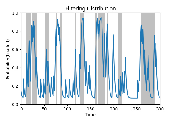
Fig. 4. Filtering for the loaded die
Figure 4 shows a graph of the posterior probabilities obtained for the loaded die. The gray background indicates the actual time periods during which this particular die was used. As can be seen from the graph, the posterior probability trajectory aligns fairly well with the actual state transitions: during periods when the loaded die is used, the probability values approach one.
Smoothing (Smoothing distribution)
Smoothing is the calculation of the posterior probabilities of a hidden state at time t, taking into account all available observations, both past and future:
p(z_t | y_{1:T})
Unlike filtering, which can be used for real-time online inference, smoothing is an offline method. It is designed to analyze historical data and also plays a key role in learning the model parameters.
This distribution is computed using the forward-backward algorithm and stored in the Sdist matrix. As with filtering, the matrix rows correspond to hidden states, and the columns correspond to time steps.
Figure 5 shows a graph of the smoothed probabilities. Because the algorithm already knows what happened in the future (at steps t + 1, t + 2, and so on) when calculating the distribution at time t, the smoothing plot appears more stable and accurate than the filtering plot, identifying the intervals when the loaded die was used with almost no errors.
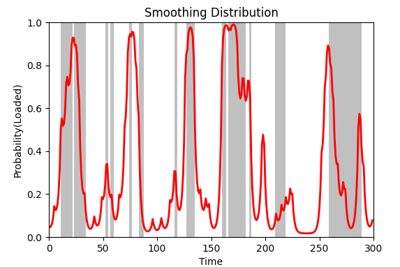
Fig. 5. Smoothed probabilities for the loaded die
So far, we have learned how to create a model, set its parameters, generate synthetic data, and perform inference by computing the filtering and smoothing distributions of the hidden states. However, in real-world problems, the true parameters of the transition and emission matrices are unknown to us. Only a sequence of observations is available. Therefore, the next step is to learn the model parameters from historical data.
Learning Model Parameters
Let's consider the joint probability distribution for the hidden and observed variables over the time interval from 1 to T:

The components of this distribution are defined as follows:
- y1:T — {y1, y2, …, yT} — a sequence of discrete observed variables,
- z1:T — {z1, z2, …, zT} — a sequence of discrete hidden states,
- p(z1) — the probability distribution of the initial hidden state (the initial vector π),
- p(zt | zt-1) — the probability of transitioning from state j at time t-1 to state k at time t (an element of the transition matrix TR),
- p(yt | zt) — the probability of obtaining a specific observation yt = i, given that the hidden variable is in state zt = k (an element of the emission matrix E).
This formula calculates the joint probability of a specific observed data trajectory and a sequence of hidden states. This factorization (decomposition of the distribution into simpler factors) is made possible by two key assumptions of the model: the Markov property (the current state remembers only the previous step) and conditional independence (an observation is generated by the current state independently of the system’s history).
We want to find the parameters θ = (TR, E) that best explain the observed data — that is, that maximize the likelihood p(y1:T∣θ). To find this likelihood, we must sum the joint probability p(y1:T, z1:T|θ) over all possible sequences of hidden states z1:T = (z1, z2, …, zT):

It is impossible to do this by brute force: even for a sequence of just 100 observations and two states, there are 2^100 hidden trajectories (combinations of state transitions). To solve this problem efficiently, we use the iterative EM (Expectation-Maximization) algorithm, which, in the context of hidden Markov models, is known as the Baum-Welch algorithm. Instead of exhaustively searching through all possible trajectories, the algorithm uses the principle of dynamic programming. In particular, the forward algorithm efficiently sums the probabilities of all possible paths at each step, computing the marginal likelihood (or its logarithm) in linear time.
//+-----------------------------------------------------------------------------+
//| Fit — Model Training (Baum-Welch Training)                                  |
//| Parameters:                                                                 |
//|   maxIter       - maximum number of iterations (100)                        |
//|   tolerance     - convergence criterion (default 1e-6)                      |
//|   verbose       - display detailed information about the training progress  |
//|                                                                             |
//| The trained parameters are stored in internal variables:                    |
//|   m_TR      — transition matrix                                             |
//|   m_E       — emission matrix                                               |
//|   m_logliks — log-likelihood history                                        |
//+-----------------------------------------------------------------------------+
bool CCategoricalHMM::Fit(const vector &y,int maxIter, double tolerance, bool verbose)
  {
   int originalL = (int)y.Size();
   int numStates = m_numStates;
   int numEmissions = m_numEmissions;

//--- Initialize the transition matrix, if not specified ---
   if(m_TR.Rows() == 0)
     {
      double default_alpha[] = {1.0}; // By default, we use the uniform Dirichlet distribution
      m_TR = RandomizeMatrix(numStates, numStates, default_alpha);
      if(verbose)
        {
         Print("TR matrix was empty, initialized with Dirichlet (alpha=1.0)");
         Print(m_TR);
         // Print(m_TR.Sum(1)); //Check that the probabilities in each matrix row sum to 1
        }
     }
   else
      if(m_TR.Rows() != numStates || m_TR.Cols() != numStates)
        {
         PrintFormat("Error: Wrong TR size. Expected %dx%d", numStates, numStates);
         return false;
        }

//--- Initialize the emission matrix if not specified ---
   if(m_E.Rows() == 0)
     {
      double default_alpha[] = {1.0};
      m_E = RandomizeMatrix(numStates, numEmissions, default_alpha);
      if(verbose)
        {
         Print("E matrix was empty, initialized with Dirichlet (alpha=1.0).");
         Print(m_E);
         // Print(m_E.Sum(1));
        }
     }
   else
      if(m_E.Rows() != numStates || m_E.Cols() != numEmissions)
        {
         PrintFormat("Error: Wrong E size. Expected %dx%d", numStates, numEmissions);
         return false;
        }

   m_logliks.Init(maxIter);
   m_logliks.Fill(0);

//--- Pseudocounts (priors) ---
   matrix pseudoTR = (m_pTR.Rows() > 0) ? m_pTR : matrix::Zeros(numStates, numStates);
   matrix pseudoE  = (m_pE.Rows() > 0)  ? m_pE  : matrix::Zeros(numStates, numEmissions);
   matrix ExpNjk = matrix::Zeros(numStates, numStates);   // E[Njk] - expected value
   matrix ExpNk = matrix::Zeros(numStates, numEmissions); // E[Nk] - expected value

   double loglik = 1.0;
   bool converged = false;

//--- Prepare the extended sequence ---
   vector seq_ext;
   seq_ext.Init(originalL + 1);
   seq_ext[0] = 0;
   for(int i = 0; i < originalL; i++)
      seq_ext[i+1] = y[i];

   int iter = 0;
   for(iter = 0; iter < maxIter; iter++)
     {
      double oldLL = loglik;
      loglik = 0;

      matrix oldGuessE = m_E;
      matrix oldGuessTR = m_TR;

      // --- Baum-Welch EM ---
      matrix Fdist, bs, Smoothing;
      vector scale;
      double logL;

      if(!Inference(y, m_TR, m_E, Smoothing, logL, Fdist, bs, scale))
         return false;

      loglik += logL;

      matrix logf = MathLog(Fdist);
      matrix logb = MathLog(bs);
      matrix logE = MathLog(m_E);
      matrix logTR = MathLog(m_TR);

      // --- Expectation Step ---
      // --- 1. XI (ξ) ---
      for(int k = 0; k < numStates; k++)
        {
         for(int j = 0; j < numStates; j++)
           {
            for(int t = 0; t < originalL; t++)
              {
               int current_obs = (int)MathRound(seq_ext[t+1]) - 1;
               //--- past (alpha)    transition      emission                future ---
               double sumLog = logf[k][t] + logTR[k][j] + logE[j][current_obs] + logb[j][t+1];
               //---  MathExp(sumLog) =  p(y1:T, zt, zt+1) ---
               //--- XI (ξ) = p(zt, zt+1 | y1:T) ---
               ExpNjk[k][j] += MathExp(sumLog) / scale[t+1]; // XI (ξ) ACCUMULATION
              }
           }
        }

      // --- 2. GAMMA (γ) ---
      for(int k = 0; k < numStates; k++)
        {
         for(int s_val = 1; s_val <= numEmissions; s_val++)
           {
            double sum_exp = 0;
            for(int t = 0; t < (int)seq_ext.Size(); t++)
              {
               if(MathRound(seq_ext[t]) == s_val) // If the symbol matches the current target symbol
                 {
                  sum_exp += MathExp(logf[k][t] + logb[k][t]); // GAMMA (γ) ACCUMULATION
                 }
              }
            ExpNk[k][s_val-1] += sum_exp;
           }
        }

      //--- Maximization step ---
      //--- Update the model parameters ---
      for(int i = 0; i < numStates; i++)
        {
         double eSum = ExpNk.Row(i).Sum(); // Update the emission matrix E
         if(eSum > 0)
            m_E.Row(ExpNk.Row(i) / eSum, i);

         double tSum = ExpNjk.Row(i).Sum(); // Update the transition matrix TR
         if(tSum > 0)
            m_TR.Row(ExpNjk.Row(i) / tSum, i);
         else
           {
            m_TR.Row(vector::Zeros(numStates), i);
            m_TR[i][i] = 1.0; // An absorbing state if there are no outgoing transitions
           }
        }

      m_logliks[iter] = loglik;

      // --- Convergence check ---
      if(verbose)
        {
         if(iter == 0)
           {
            Print("Log Likelihood and Relative Changes in Log Likelihood, Transition Matrix and Emission Matrix");
            Print("   Iteration      LogLik      Log Lik Rel     Transition      Emission");
           }
         else
           {
            double relLL = MathAbs(loglik - oldLL) / (1.0 + MathAbs(oldLL));
            double relTR = (m_TR - oldGuessTR).Norm(MATRIX_NORM_INF) / numStates;
            double relE = (m_E - oldGuessE).Norm(MATRIX_NORM_INF) / numEmissions;
            PrintFormat("     %6d   %12g   %12g  %12g  %12g", iter + 1,loglik, relLL, relTR, relE);
           }
        }

      if(iter > 0 && (MathAbs(loglik - oldLL) / (1.0 + MathAbs(oldLL))) < tolerance)
        {
         if((m_TR - oldGuessTR).Norm(MATRIX_NORM_INF) / numStates < tolerance &&
            (m_E - oldGuessE).Norm(MATRIX_NORM_INF) / numEmissions < tolerance)
           {
            converged = true;
            if(verbose)
               PrintFormat("Converged after %d iterations.", iter + 1);
            break;
           }
        }
      //--- Reset to pseudocounts or zero if pseudocounts are not used ---
      ExpNjk = pseudoTR;
      ExpNk  = pseudoE;
     }

   if(!converged)
     {
      if(verbose)
        {
         PrintFormat("Algorithm did not converge with tolerance %g in %d iterations.",tolerance, maxIter);
        }
     }

   m_logliks.Resize(iter < maxIter ? iter + 1 : maxIter); // Remove unused trailing entries from logliks

   return true;
  }
The algorithm works by iteratively performing two steps:
1. E-step (Expectation)
In this step, the parameters of the matrices m_TR and m_E are held fixed (in the first iteration, they are initialized with random values drawn from a Dirichlet distribution or specified by the user). The forward-backward algorithm is used to calculate conditional posterior probabilities that serve as sufficient statistics:
XI ξt(k, j) — the probability of transitioning from state k to state j at time t, given the entire observation sequence:
where
- p(zt | y1:t) — filtering (forward variable) logf[k][t],
- p(zt+1 | zt) — an element of the transition matrix logTR[k][j],
- p(yt+1 | zt+1) — the local likelihood of the new observation, an element of the emission matrix logE[j][current_obs],
- p(yt+2:T | zt+1) — backward variable logb[j][t+1]
Gamma (γ) — the probability that the system is in a particular state at each step, given the entire observation history (smoothed distribution/smoothing)
These probabilities are used to accumulate expected event frequencies:
- The ExpNjk matrix accumulates the expected number of transitions between states,
- The ExpNk matrix accumulates the expected frequency of occurrence of each symbol in each state.
Thus, instead of actual (but unknown) states, the algorithm operates on their probability weights.
2. M-step (Maximization)
In this step, the model parameters are updated based on the calculated sufficient statistics. Transition and emission matrices are recalculated by normalizing the rows: the accumulated weighted frequency is divided by the total sum for that row.
If, for any state, the sum of outgoing transitions is zero, that state is automatically converted to an absorbing state (a value of 1.0 is set on the main diagonal).
The cycle (Calculate probabilities using the old matrices → Update the matrices using the new probabilities) repeats until the relative changes in log-likelihood (relLL) and the matrix parameters (relTR, relE) all fall below the user-specified tolerance.
To test the algorithm, let's generate the same sequence used in the example with Inference.mql5 and try to recover the original TR and E parameter matrices (the Learning.mql5 script).
//+------------------------------------------------------------------+
//|                                                     Learning.mq5 |
//|                                                           Eugene |
//|                                             https://www.mql5.com |
//+------------------------------------------------------------------+
#property copyright "Eugene"
#property link      "https://www.mql5.com"
#property version   "1.00"
#include <CategoricalHMM\CategoricalHMM.mqh>
#include <Graphics\Graphic.mqh>
//+------------------------------------------------------------------+
//| Script program start function                                    |
//+------------------------------------------------------------------+
void OnStart()
  {
   int n_states = 2;
   int n_emissions = 6;
   int n_samples = 300;

//--- 1. Create a model (seed=99 for reproducibility) ---
   CCategoricalHMM model(n_states, n_emissions, 99);

// --- Set the model parameters ---
// --- 2. Set the transition matrix (Tr) ---
   matrix tr = {{0.95, 0.05},
        {0.1,  0.9}
     };

// --- 3. Set the emission matrix (E) ---
   matrix e = {{1.0/6, 1.0/6, 1.0/6, 1.0/6, 1.0/6, 1.0/6},
        {0.1,   0.1,   0.1,   0.1,   0.1,   0.5}
     };

// --- 4. Generate a sequence of observations and hidden states ---
   vector y,z;
   model.Sample(n_samples, tr, e, y, z);

// --- 5. Create a new model and train it on the generated data ---
   CCategoricalHMM hmm(n_states, n_emissions);
// --- Set the following initial parameters: ---
   matrix initialTR = {{0.7, 0.3},
        {0.3, 0.7}
     };
   matrix initialE  = {{0.15, 0.05, 0.1, 0.1, 0.4, 0.2},
        {0.05, 0.15, 0.1, 0.1, 0.3, 0.3}
     };

   hmm.m_TR = initialTR;
   hmm.m_E = initialE;

   double tol = 1e-6;
   if(hmm.Fit(y,100, tol, true))
     {
      Print("\n--- Results ---");
      PrintFormat("Final LogLikelihood: %.6f", hmm.m_logliks[hmm.m_logliks.Size() - 1]);
      Print("Estimated TR:\n", hmm.m_TR);
      Print("True TR:\n", tr);
      Print("Estimated E:\n", hmm.m_E);
      Print("True E:\n", e);
     }

// --- VISUALIZATION SECTION ---
   int plotLimit = (int)hmm.m_logliks.Size();
   double x[], y_[];
   ArrayResize(x, plotLimit);
   ArrayResize(y_, plotLimit);
   for(int i = 0; i < plotLimit; i++)
     {
      x[i] = i;
      y_[i] = hmm.m_logliks[i];
     }
   ChartSetInteger(0,CHART_SHOW,false);
   CGraphic graphic;
   ulong width = ChartGetInteger(0,CHART_WIDTH_IN_PIXELS);
   ulong height = ChartGetInteger(0,CHART_HEIGHT_IN_PIXELS);
   graphic.Create(0,"HMM_States_Plot",0,0,0,int(width),int(height));
   CCurve *curve = graphic.CurveAdd(x, y_, ColorToARGB(clrDodgerBlue, 255), CURVE_LINES,"LL");
   curve.LinesStyle(STYLE_SOLID);
   curve.LinesWidth(2);
   graphic.BackgroundMainColor(ColorToARGB(clrBlack,255));
   graphic.BackgroundMainSize(24);
   graphic.BackgroundMain("EM Training Progress");
   graphic.XAxis().Name("Iteration");
   graphic.XAxis().NameSize(18);
   graphic.YAxis().Name("Log Likelihood");
   graphic.YAxis().NameSize(18);
   graphic.CurvePlotAll();
   graphic.Update();
   Sleep(5*1000);
   ChartSetInteger(0,CHART_SHOW,true);
   graphic.Destroy();
   ChartRedraw(0);
  }
//+------------------------------------------------------------------+
To ensure the reproducibility of the results in this experiment, we explicitly specify the initial approximation matrices initialTR and initialE.
In real-world problems, if the initial parameters are not specified, the Fit() method automatically initializes them using a Dirichlet distribution. If you want to use automatic random initialization but maintain reproducibility of results from run to run, be sure to pass a fixed seed value greater than 0 to the constructor of the CCategoricalHMM class.
Let's compare the parameters recovered by the algorithm with their true values:
        Estimated TR:
        [[0.960567347171196,0.03943265282880401]
         [0.1389165412495843,0.8610834587504157]]
        True TR:
        [[0.95,0.05]
         [0.1,0.9]]
        Estimated E:
        [[0.1796760822470783,0.1183101172299737,0.2125226716621954,0.1291808115499933,0.1924550232457491,0.1678552940650102]
         [2.431736724262778e-19,0.1712486186920382,0.09543183463784231,0.02722383599510184,0.03038479513837311,0.6757109155366445]]
        True E: [[0.1666666666666667,0.1666666666666667,0.1666666666666667,0.1666666666666667,0.1666666666666667,0.1666666666666667]
         [0.1,0.1,0.1,0.1,0.1,0.5]]
As we can see, on the whole, the results obtained are very close to the true values of the parameters. The model determined that the first hidden state generates symbols relatively uniformly, while the second has a bias toward the number 6 (probability 0.675 versus the true probability of 0.5). Of course, when analyzing accuracy, it is necessary to account for the small sample size — only 300 observations. Nevertheless, even with such a small dataset, the algorithm demonstrated good convergence.
Figure 6 shows the learning curve — a graph of changes in the log-likelihood. The specified accuracy level, tolerance = 1e-6, was successfully achieved in 88 iterations.
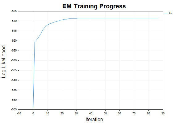
Fig. 6. Marginal likelihood learning curve
In conclusion, we note once again that the EM algorithm guarantees convergence only to a local maximum of the objective function (likelihood) and is extremely sensitive to the initialization. To find the global optimum and obtain the most stable estimates, it is recommended to use a multi-start strategy. This strategy involves running the training process several times with different random initial values for the matrix parameters, then selecting the model with the highest log-likelihood.
Selecting the Optimal Number of Hidden States (Model Selection)
In practice, when working with real market quotes, we never know the true data-generating process. This naturally raises the question: How many hidden states should be specified for the model? If there are too few states, the model will not be able to describe the complex data structure (underfitting). If there are too many states, the model will begin to fit random noise (overfitting), completely losing its predictive ability.
To answer this question, information criteria are traditionally used in mathematical statistics:
- AIC (Akaike Information Criterion),
- BIC (Bayesian Information Criterion).
Both criteria strike a balance between the quality of the model fit and its complexity, penalizing an increase in the number of parameters. The model with the lowest AIC or BIC value is considered optimal.
Let us examine the model selection process (the ModelSelection.mq5 script).
//+------------------------------------------------------------------+
//|                                               ModelSelection.mq5 |
//|                                                           Eugene |
//|                                             https://www.mql5.com |
//+------------------------------------------------------------------+
#property copyright "Eugene"
#property link      "https://www.mql5.com"
#property version   "1.00"
#include <CategoricalHMM\CategoricalHMM.mqh>
#include <Graphics\Graphic.mqh>
//+------------------------------------------------------------------+
//| Script program start function                                    |
//+------------------------------------------------------------------+
void OnStart()
  {
   int n_samples = 5000;
   int n_states_true = 3;
   int n_emissions = 6;

// --- 1. INITIALIZATION OF THE TRUE MODEL FOR GENERATION ---
   matrix tr_true =
     {
        {0.8, 0.1, 0.1},
        {0.05, 0.9, 0.05},
        {0.1, 0.1, 0.8}
     };

   matrix e_true =
     {
        {1.0/6, 1.0/6, 1.0/6, 1.0/6, 1.0/6, 1.0/6},
        {0.1, 0.1, 0.1, 0.1, 0.1, 0.5},
        {0.4, 0.1, 0.1, 0.1, 0.1, 0.2}
     };

   vector y, states_true;
   CCategoricalHMM gen_model(n_states_true, n_emissions, 42); // Seed 42
   gen_model.Sample(n_samples, tr_true, e_true, y, states_true);
//VectorToCSV("Sample5000.csv", y);

// --- CALCULATION OF THE TRUE LOG-LIKELIHOOD ---
   double true_ll = 0;
   matrix p_true, fs_true, bs_true;
   vector s_true;

// --- Calling Inference with the true parameters ---
   gen_model.Inference(y, tr_true, e_true, p_true, true_ll, fs_true, bs_true, s_true);

   PrintFormat("==================================================");
   PrintFormat("TRUE MODEL LOG-LIKELIHOOD: %.2f", true_ll);
   PrintFormat("==================================================");

// --- 2. MODEL SELECTION ---
   int ns[] = {1,2, 3, 4, 5, 6, 7};
   int n_fits = 10;
   int n_points = ArraySize(ns);
   double x_vals[], aic_vals[], bic_vals[]; // Arrays for the plot
   ArrayResize(x_vals, n_points);
   ArrayResize(aic_vals, n_points);
   ArrayResize(bic_vals, n_points);

   Print("==================================================");
   Print("HMM MODEL SELECTION ");
   PrintFormat("True States: %d | Samples: %d", n_states_true, n_samples);
   Print("==================================================");

   for(int i = 0; i < ArraySize(ns); i++)
     {
      int n_curr = ns[i];
      double best_ll = -DBL_MAX;
      int n_params;

      // --- Try several random starts for each N ---
      for(int fit = 0; fit < n_fits; fit++)
        {
         CCategoricalHMM model(n_curr, n_emissions, fit);
         n_params = model.GetParams();

         // --- Train (20 iterations for a quick evaluation) ---
         if(!model.Fit(y, 20, 1e-4,false))
            continue;

         // --- Obtain the log-likelihood ---
         double current_ll = 0;
         matrix p, fs, bs;
         vector s;
         if(model.Inference(y, model.m_TR, model.m_E, p, current_ll, fs, bs, s))
           {
            if(current_ll > best_ll)
               best_ll = current_ll;
           }
        }

      // --- Evaluate information criteria for the best run at the current N ---
      CCategoricalHMM eval_model(n_curr, n_emissions);
      double val_aic = eval_model.AIC(best_ll);
      double val_bic = eval_model.BIC(best_ll, n_samples);

      // --- Save data for the plot ---
      x_vals[i] = n_curr;
      aic_vals[i] = val_aic;
      bic_vals[i] = val_bic;

      PrintFormat("N=%d | LL: %.2f | AIC: %.2f | BIC: %.2f | n_params:%d",
                  n_curr, best_ll, val_aic, val_bic,n_params);
     }
   Print("==================================================");

// --- VISUALIZATION ---
   ChartSetInteger(0, CHART_SHOW, false);

   CGraphic graphic;
   ulong width = ChartGetInteger(0, CHART_WIDTH_IN_PIXELS);
   ulong height = ChartGetInteger(0, CHART_HEIGHT_IN_PIXELS);

   if(ObjectFind(0, "HMM_Selection_Plot") < 0)
      graphic.Create(0, "HMM_Selection_Plot", 0, 0, 0, int(width), int(height));
   else
      graphic.Attach(0, "HMM_Selection_Plot");

   CCurve *curveAIC = graphic.CurveAdd(x_vals, aic_vals, ColorToARGB(clrDodgerBlue, 255), CURVE_POINTS_AND_LINES, "AIC");
   curveAIC.LinesStyle(STYLE_SOLID);

   CCurve *curveBIC = graphic.CurveAdd(x_vals, bic_vals, ColorToARGB(clrLimeGreen, 255), CURVE_POINTS_AND_LINES, "BIC");
   curveBIC.LinesStyle(STYLE_SOLID);

   graphic.BackgroundMainColor(ColorToARGB(clrBlack, 255));
   graphic.BackgroundMainSize(24);
   graphic.BackgroundMain("HMM Model Selection (AIC vs BIC)");
   graphic.XAxis().Name("Number of States");
   graphic.XAxis().NameSize(18);
   graphic.YAxis().Name("AIC/BIC Value (Lower is Better)");
   graphic.YAxis().NameSize(18);
   graphic.CurvePlotAll();
   graphic.Update();
   Sleep(10000);
   ChartSetInteger(0, CHART_SHOW, true);
   graphic.Destroy();
   ChartRedraw(0);
  }
//+------------------------------------------------------------------+
Let's generate a sample of 5,000 observations from a known HMM with three states (N = 3):
- State 1 (Fair die): Uniform distribution over the faces (1/6),
- State 2 (Asymmetry): Biased toward rolling sixes (0.5),
- State 3 (Asymmetry): Biased toward rolling ones (0.4).
Next, we will train 7 different HMM architectures in sequence (with the number of states N ranging from 1 to 7). To reduce the impact of local maxima, each architecture is trained 10 times (n_fits = 10) using random starting points. The run with the highest log-likelihood (LL) is selected as the final result. The number of training iterations was limited to 20 to speed up the experiment.
As the number of states increases, the log-likelihood increases as expected:
- Single-state model (N=1): reduces the transition matrix to a 1×1 matrix with a single entry of 1.0, completely eliminating regime-switching dynamics. The emission matrix becomes an ordinary frequency vector. The model simply estimates the baseline probabilities of rolling each face across the entire dataset, requiring just one training iteration (LL = −8425.95).
- Transition to two states (N=2): there is virtually no noticeable improvement (LL = −8,422.48).
- Transition to three states (N=3): there is a significant increase in LL from −8,422 to −8,397. This indicates that this model better explains the data.
- Further increases in the number of states (N ≥ 4): the log-likelihood generally continues to increase (as shown in Fig. 7), since the additional parameters allow a closer fit to random fluctuations in the sample.
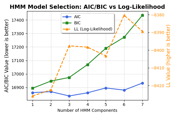
Fig. 7. Information criteria and log-likelihood for different numbers of hidden states
However, relying solely on maximum likelihood leads directly to overfitting. Otherwise, we would simply choose the model with 6 hidden states. Now let's examine the results obtained using information criteria (Fig. 8).
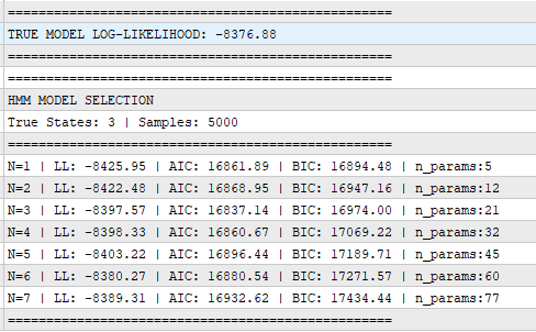
Fig. 8. Best AIC/BIC and LL results for 7 models
The AIC clearly indicates a minimum at the true value of N=3 (AIC = 16,837.14), confirming its ability to identify the actual complexity of the process. The BIC, on the other hand, favors the simplest model (N=1; BIC = 16,894.48), ranking the true model (N=3) only third. There are two reasons for this discrepancy:
First, BIC imposes a heavier penalty: its penalty per parameter scales as ln(T), where T is the sample size. With 5,000 observations, the penalty for each additional parameter is approximately 8.51. Moving from a 1-state model to a 3-state model adds 16 parameters. The increase in the log-likelihood was insufficient to compensate for such a significant increase in the model's complexity.
Second, the training was incomplete — the 20-iteration limit prevented the models with N=3 from fully converging to a local optimum. The true model has LL ≈ −8376.88, whereas the best of the trained models achieves only LL ≈ −8397.57. The difference of nearly 21 points had a significant impact on the final values of the criteria.
Nevertheless, the main conclusion remains clear: when choosing an HMM architecture, one should not simply pursue the highest likelihood. The correct approach is to use the AIC and BIC information criteria, which help strike a reasonable balance between goodness of fit and model complexity.
Online Filtering of Hidden States and the Bayesian Filter
Online filtering in the context of hidden Markov models is the process of recursively updating the probabilities of hidden states in real time as new observations are received. Unlike offline methods (such as smoothing), which perform a batch analysis of the entire sample at once, online filtering operates sequentially over time (t = 1, 2, 3, …, T).
The main task of online filtering is to compute the current posterior distribution P(zt | y1:t). This process is implemented recursively and consists of two phases at each time step:
- Prediction step — calculation of the prior distribution,
- Filtering step (Update) — correction of the prediction using a new observation via Bayes' theorem (calculation of the posterior distribution).
In an HMM, Bayes' theorem for the online filtering step takes the following form:

where
- The posterior probability p(z_t = j | y_{1:t}) is the updated (filtered) probability that the system is in state j at time t, given the entire available observation history, including the latest observation y_t,
- The local likelihood p(y_t | z_t = j) is an element of the emission matrix (E) that represents the probability of generating the symbol y_t given that the system is in hidden state j,
- The prior probability (prediction step) p(z_t = j | y_{1:t-1}) is the predicted state distribution at step t, based on information from the previous step (t−1). It is calculated by multiplying the previous filtering distribution by the transition matrix.

- The marginal likelihood (evidence) p(y_t | y_{1:t-1}) is the total probability of observing y_t given the current model parameters. This is a normalizing constant that ensures that the sum of the probabilities of all states at the current step equals 1.
To demonstrate the online filtering process, consider the Filter.mql5 script.
//+------------------------------------------------------------------+
//|                                                       Filter.mq5 |
//|                                                           Eugene |
//|                                             https://www.mql5.com |
//+------------------------------------------------------------------+
#property copyright "Eugene"
#property link      "https://www.mql5.com"
#property version   "1.00"
#include <CategoricalHMM\CategoricalHMM.mqh>
//+------------------------------------------------------------------+
//| Script program start function                                    |
//+------------------------------------------------------------------+
void OnStart()
  {
//--- 1. Model parameters ---
   matrix tr = {{0.95, 0.05},
        {0.10, 0.90}
     };
   matrix e = {{0.16, 0.16, 0.16, 0.16, 0.16, 0.20},
        {0.10, 0.10, 0.10, 0.10, 0.10, 0.50}
     };
   vector y = {1, 6, 6, 6, 2}; // Sequence of observations

   CCategoricalHMM hmm(2, 6);
   hmm.m_TR = tr;
   hmm.m_E = e;

//--- Initial state ---
   vector currentFilterState = {1.0, 0.0};
   vector cfs = currentFilterState;
   Print("=== CONSECUTIVE ONLINE FORECAST ===");

   for(int i = 0; i < (int)y.Size(); i++)
     {
      int obs = (int)y[i];

      // --- STEP 1: PREDICTION (before the current observation is known) ---
      vector statePrediction = currentFilterState @ hmm.m_TR;
      PrintFormat("Time t=%d:", i+1);
      PrintFormat("  State forecast : [1]%.4f, [2]%.4f", statePrediction[0], statePrediction[1]);

      vector obsPrediction = statePrediction @ hmm.m_E; // Multiply the predicted state distribution by the emission matrix

      ulong maxObsIdx = obsPrediction.ArgMax(); // Find the most likely observation
      PrintFormat("  The most probable next observation: %d (with the probability of %.4f)", maxObsIdx + 1, obsPrediction[maxObsIdx]);

      // --- STEP 2: UPDATE (FILTERING) ---
      // --- Observation obs has arrived; update the current state ---
      currentFilterState = hmm.Filter(currentFilterState, obs);

      PrintFormat("  REALITY: %d observation has been received. Current state updated (Filtering): [1]%.4f, [2]%.4f",
                  obs, currentFilterState[0], currentFilterState[1]);
      Print("---------------------------------------");
     }

// --- OPTION 1: SEQUENTIAL (online) ---
   Print("=== 1. ONLINE FILTER (STEP-BY-STEP) ===");
   currentFilterState = cfs;
   for(int i = 0; i < (int)y.Size(); i++)
     {
      currentFilterState = hmm.Filter(currentFilterState, (int)y[i]);
      PrintFormat("Time t = %d (after y = %d): [1]%.4f, [2]%.4f", i+1, (int)y[i], currentFilterState[0], currentFilterState[1]);
     }

// --- OPTION 2: BATCH (inference) ---
   Print("\n=== 2. BATCH Inference (Filtering Distribution) ===");
   matrix pStates, fs, bs;
   vector s_vec;
   double logP;

   if(hmm.Inference(y, tr, e, pStates, logP, fs, bs, s_vec))
     {
      PrintMatrixFormatted(fs,4);
     }
  }

//-------------Script Execution Results ----------------------

// === SEQUENTIAL ONLINE PREDICTION ===
// Time t = 1:
//   State forecast: [1]0.9500, [2]0.0500
//   Most likely next observation: 6 (with a probability of 0.2150)
//   REALITY: Observation 1 has been received. Current state updated (Filtering): [1]0.9682, [2]0.0318
// ---------------------------------------
// Time t = 2:
//   State forecast: [1]0.9229, [2]0.0771
//   Most likely next observation: 6 (with a probability of 0.2231)
//   REALITY: Observation 6 has been received. Current state updated (Filtering): [1]0.8273, [2]0.1727
// ---------------------------------------
// Time t = 3:
//   State forecast: [1]0.8032, [2]0.1968
//   Most likely next observation: 6 (with a probability of 0.2590)
//   REALITY: Observation 6 has been received. Current state updated (Filtering): [1]0.6201, [2]0.3799
// ---------------------------------------
// Time t = 4:
//   State forecast: [1]0.6271, [2]0.3729
//   Most likely next observation: 6 (with a probability of 0.3119)
//   REALITY: Observation 6 has been received. Current state updated (Filtering): [1]0.4022, [2]0.5978
// ---------------------------------------
// Time t = 5:
//   State forecast: [1]0.4418, [2]0.5582
//   Most likely next observation: 6 (with a probability of 0.3674)
//   REALITY: Observation 2 received. Current state updated (Filtering): [1]0.5588, [2]0.4412
// ---------------------------------------
// === 1. ONLINE FILTER (STEP-BY-STEP) ===
// Step t = 1 (after y = 1): [1]0.9682, [2]0.0318
// Step t = 2 (after y = 6): [1]0.8273, [2]0.1727
// Step t = 3 (after y = 6): [1]0.6201, [2]0.3799
// Step t = 4 (after y = 6): [1]0.4022, [2]0.5978
// Step t = 5 (after y = 2): [1]0.5588, [2]0.4412
//
// === 2. BATCH Inference (Filtering Distribution) ===
//   1.0000 0.9682 0.8273 0.6201 0.4022 0.5588
//   0.0000 0.0318 0.1727 0.3799 0.5978 0.4412
We assume that the model has already been trained and that the transition matrix (TR) and emission matrix (E) are known. The script simulates real-time data input using the following sequence as an example: y = {1, 6, 6, 6, 2}.
Processing each time interval involves two steps:
- Prediction step (before the current bar t closes): We multiply the state distribution vector from the previous step, currentFilterState, by the transition matrix (at step t=1, the vector is initialized with the initial probabilities, for example, {1.0, 0.0}). The hidden state prediction is calculated before the current bar closes and a new observation is received. Additionally, at this stage, you can calculate which specific observation (which outcome) is most likely on the current bar.
- Filtering step (after bar t closes): As soon as the bar closes, we obtain the actual observation value y. Using Bayes' formula, the model performs an update — it refines the probabilities of states at the current time t based on this observation.
- Transition to step t+1: The resulting posterior vector serves as the basis for the next step. We use this vector to make a prediction for time t+1, and the system then waits for a new observation.
The cycle (forecast → bar close → filtering → forecast for the next step) is repeated for each new observation {t+1, t+2, …}, updating the hidden-state estimate online.
Note that the values obtained through online filtering match exactly the columns of the Fdist matrix returned by the Inference() method during batch processing. This confirms that the implementation is correct: regardless of whether data is fed in batches or as a stream, the same forward-pass algorithm is used.
Conclusion
In this article, we have provided a detailed analysis of the theoretical foundations and practical implementation of hidden Markov models with categorical emissions (Categorical HMMs) in the MQL5 language. In the course of our research, we systematically examined the key problems that the model addresses: - inference of hidden states (the Inference method) — calculation of posterior distributions based on a scaled forward-backward algorithm,
- parameter learning (the Fit method) — an iterative EM algorithm that includes stochastic initialization of matrices using the Dirichlet distribution and regularization using prior pseudocounts,
- model selection — selecting the optimal number of hidden states using the AIC and BIC information criteria, which protect the model from overfitting,
- online filtering (the Filter method) — a recursive Bayesian filter that allows the probabilities of hidden states to be updated in real time as new data arrives.
The categorical model provides traders with a rigorous mathematical tool for identifying hidden states based on observable variables. Understanding how this model works lays a solid foundation for further study and the development of more complex state-space models.
Software used in this article
| # | Name | Type | Description |
|---|---|---|---|
| 1 | CategoricalHMM.mqh | Class | Categorical hidden Markov model class |
| 2 | Inference.mq5 | Script | Example of inferring hidden states and generating synthetic data from a given model |
| 3 | Learning.mq5 | Script | Example of training a model |
| 4 | ModelSelection.mq5 | Script | Example of selecting the optimal number of hidden states using the AIC/BIC criteria |
| 5 | Filter.mq5 | Script | Example of building a recursive Bayesian filter |
| 6 | MQL5.zip | Archive | Find all of the files listed above in the MQL5 archive |
Translated from Russian by MetaQuotes Ltd.
Original article: https://www.mql5.com/ru/articles/22745
Warning: All rights to these materials are reserved by MetaQuotes Ltd. Copying or reprinting of these materials in whole or in part is prohibited.
This article was written by a user of the site and reflects their personal views. MetaQuotes Ltd is not responsible for the accuracy of the information presented, nor for any consequences resulting from the use of the solutions, strategies or recommendations described.



Thank you for your feedback.
You see, filtering and a moving average are completely different things. A moving average is simply an average calculated over a sliding window. Filtering is the process of calculating the probability distribution of hidden states. It is a set of probabilities. In other words, it is an assessment of the state we are in at the current moment in time. If the probability is higher for an uptrend, it means the market is most likely in that state, and you can then open a position in line with the trend. If the probability of being in a state of noise (a 50/50 chance of a white candle) is higher, it means the market is currently random and opening trades is not recommended. That is the main idea. Therefore, if you use moving averages to determine an entry point, the HMM acts as a safeguard that will prevent you from opening a trade if it determines that there is no trend at the moment.
But before implementing the trading algorithm, we need to detect these hidden states. How can we do this if we only have a dataset? Using a learning algorithm (EM). It’s like finding parameters in an MLP via gradient descent. By analysing the parameters obtained, we can conclude whether any hidden states are present in the data at all, or whether the market is in a state of chaos and there is only one mode (equal emission probabilities for each state).
Train the model for the coin-toss scenario (white/black candlestick) for two states (fair/biased); you will then be able to better understand the model’s capabilities.