MCMC Sampling Methods — The Metropolis-Hastings Algorithm

Introduction

Markov chain Monte Carlo (MCMC) methods are a class of sampling algorithms that allow one to draw samples from a complex target distribution p(x). The goal of MCMC is to obtain a set of samples that accurately represent this target distribution so that the means, variances, and other characteristics of this distribution can be estimated. MCMC is based on constructing a Markov chain whose stationary distribution coincides with the target distribution.

These methods are widely used in Bayesian inference, machine learning, and other fields where approximations of posterior distributions are required. Unlike deterministic methods such as variational inference or Laplace approximation, MCMC algorithms have a unique property: when properly configured, they are guaranteed in the limit to produce samples that exactly match the target distribution. Among the many MCMC algorithms, the Metropolis-Hastings (MH) algorithm holds a special place — it is a fundamental method that underlies many modern approaches.

In this article, we will examine the Metropolis-Hastings algorithm, starting with its theoretical foundations and key concepts. Next, we will present an implementation of the algorithm in MQL5 as the MHSampler class, and we will also examine simple examples of its application to univariate and multivariate distributions, including the Random Walk and Independent MH variants.

It should be noted that when using MCMC methods, special attention should be paid to diagnosing and tuning the algorithm, since its correct operation requires a thorough analysis of the chain’s convergence using statistical and visual tools.

The Metropolis Algorithm

The basic Metropolis algorithm (Metropolis, 1953) generates samples from the target distribution by proposing, at each step, a transition from the current state x to a new state x′ with probability q(x′∣x), where q is called the proposal distribution. The main requirement for the proposal distribution is that it must ensure that the chain does not get stuck in a single region; in other words, it must be possible to move from any point in the support of the target distribution to any other point. For this, it suffices that the probability q(x′∣x) be nonzero for all possible states x and x′.

The proposed state x′ is accepted or rejected based on a criterion that ensures the chain visits states in the long run in proportion to p(x). If state x′ is accepted, it becomes the new state; otherwise, the chain remains in its current state (the sample is duplicated).

The Metropolis algorithm is a special case of the Metropolis-Hastings algorithm in which the proposal distribution q(x′∣x) is symmetric; that is, the probability of proposing the forward transition from x to x′ is equal to the probability of the reverse transition: q(x′∣x) = q(x∣x′).

Thanks to this symmetry, the acceptance criterion for the candidate x′ is greatly simplified:

A = min(1, p*(x')/p*(x))

where p*(x) is the unnormalized density of the target distribution, and the distribution itself is defined as p(x) = p*(x)/Zp.

The normalization constant Zp may be unknown, which makes the algorithm particularly useful for problems where it is difficult to compute Zp analytically, as is often the case in Bayesian inference.

If the density at the new point x′ is higher than at the current point x (i.e., p*(x′) > p*(x)), then the acceptance probability A = 1, and the transition to x′ always occurs (with probability 1). This allows the chain to quickly climb toward the peaks of the distribution, helping it find regions of high probability.

If the density decreases (p*(x′) < p*(x)), the transition to x′ occurs with probability A = p*(x′)/p*(x). This mechanism allows the chain to descend from the peaks of the distribution and explore its slopes and valleys, ensuring efficient exploration of the entire space and preventing the chain from getting permanently stuck at a single point.

It is precisely this balance between unconditional acceptance of “uphill” moves and probabilistic acceptance of “downhill” moves that ensures the chain preserves the proportions of the target distribution by spending more time where the density is higher.

The sequence of samples obtained in this way forms a Markov chain, in which each subsequent state depends on the previous one. This leads to autocorrelation among the samples, which can reduce their representativeness (because of high autocorrelation, adjacent samples contain nearly identical information).

For example, if you have collected 1,000 highly correlated samples, they may contain the same information as just 50 independent samples. Your 1,000 samples do not represent 1,000 unique observations of the distribution; they provide only 50 effective observations. As a result, estimates of the mean, variance, and other characteristics of the distribution based on these correlated samples will have a higher variance (error) than if you had used the same number of independent samples. Therefore, to reduce autocorrelation, a so-called burn-in period — which discards the initial iterations — and thinning — which retains only every i-th sample — are used.

Fig. 1. Metropolis algorithm

Markov Chains

Markov chain Monte Carlo methods use Markov chains to generate samples from complex distributions. To understand how this works, let us examine two key properties of Markov chains that must hold in order to construct an MCMC algorithm: their “memory” and their ability to converge to the desired distribution.

1. Markov property

A Markov chain is a sequence of states x(1), x(2), … in which each subsequent state x(t+1) depends only on the current state x(t) and does not depend on the entire previous history of the chain x(1), …, x(t−1):

P(x(t+1) | x(t), …, x(1)) = P(x(t+1) | x(t))

This property means that knowing only the present is sufficient to predict the future state.

2. Convergence to the target distribution

The goal of MCMC algorithms is to construct a Markov chain that, over time (after an initial burn-in period), generates samples from the target distribution p(x). This is achieved through a special transition rule that satisfies the detailed balance condition (Detailed Balance):

p(x)T(x′∣x) = p(x′)T(x∣x′)

where:

• p(x) and p(x′) are the densities of the target distribution,
• T(x′∣x) is the total transition probability from x to x'.

In the Metropolis-Hastings algorithm, this important condition is ensured by choosing an appropriate acceptance probability A, which guarantees that, over time, the chain “visits” states in proportion to p(x), even if the distribution itself is specified only up to a normalizing constant (without the normalizing constant Zp). In this case, the total transition probability T(x′∣x) is constructed as the product of the proposal probability q(x′∣x) and the acceptance probability A(x′∣x).

Metropolis-Hastings Algorithm

The Metropolis-Hastings algorithm (Hastings, 1970) generalizes the Metropolis algorithm, allowing asymmetric proposal distributions to be used, that is, q(x′|x) ≠ q(x|x′). This makes the algorithm more flexible and applicable to a wide class of problems where symmetric distributions are not suitable (for example, when using lognormal or exponential proposals).

To compensate for asymmetry, the Hastings correction is introduced into the acceptance criterion A; it corrects the bias created by an asymmetric proposal distribution. The acceptance probability for candidate x' is defined as:

A = min(1, p*(x')q(x|x') / p*(x)q(x'|x))

where:

• p*(x) — the unnormalized density of the target distribution,
• q(x|x') / q(x'|x) — the Hastings correction, which accounts for the asymmetry of the proposal distribution.

As before, calculating A does not require knowledge of the normalizing constant Zp in the probability density p(x) = p*(x)/Zp, since it cancels out.

Effect of the Proposal Distribution on Performance

The choice of q(x'|x) significantly affects the algorithm's efficiency. In continuous spaces, a normal distribution centered at the current state x(t) is often used, resulting in behavior known as Random Walk Metropolis-Hastings (RWMH). In this context, the variance parameter (or step size) plays a key role, as it determines the scale of the proposed transitions:

• Low variance: The acceptance rate will be high, but the chain will move slowly. This will result in long autocorrelation times for the samples, since the chain explores the space slowly.
• High variance: The acceptance rate will be low, since most of the proposed moves will fall into low-probability regions. This leads to frequent rejections and inefficient use of computational resources.

In practice, optimal performance is achieved when the acceptance rate is in the 20–40% range. This requires careful tuning of the parameters of q to balance the speed of exploration of the space against the acceptance probability.

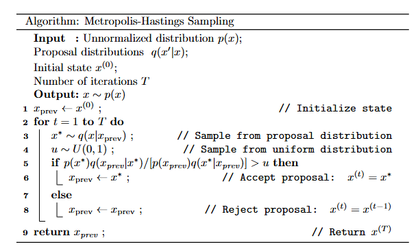
Fig. 2. Metropolis-Hastings Algorithm

The Metropolis-Hastings algorithm has been implemented in MQL5 using an object-oriented approach. The main MHSampler class requires the implementation of three abstract classes: LogPDF (target log-density), PropRND (new-state generator), and LogPropPDF (proposal transition log-density). This makes it easy to adapt the algorithm for any target and proposal distribution.

The LogPDF class

The LogPDF class defines an interface for computing the log-density of the target distribution p*(x). The LogPdf(const vector &x) method takes a vector x (a point in the state space) and returns ln p*(x).

Using the logarithm of the density is standard practice in MCMC, as it prevents numerical errors when dealing with small probabilities, especially in multivariate problems. The class can be implemented for any target distribution, such as a normal distribution or a mixture of distributions. In Bayesian inference, this class is implemented to compute the logarithm of the unnormalized posterior density, which is expressed as the sum of logarithms: ln p*(x) = ln(likelihood) + ln(prior distribution).

The PropRND class

The PropRND class is responsible for generating random candidate states x′ from the proposal distribution q(x′∣x). The PropRnd(const vector &x) method takes the current state x and returns a new vector x′ generated from the proposal distribution q(x′∣x).

For example, for random-walk MH, the user can implement PropRND using a Gaussian distribution centered at the current state x, and for independent MH, using a fixed distribution that does not depend on x.

The LogPropPDF class

The LogPropPDF class is responsible for computing the log-density of the proposal distribution q(x′∣x). This class does not generate new states; it only evaluates the transition probability density. The LogPropPdf(const vector &x_to, const vector &x_from) method returns ln q(x′∣x), where x′ is the proposed new state and x is the current state.

This class is used only for asymmetric proposal distributions. In such cases, ln⁡q(x'∣x) is needed to compute the Hastings correction in the acceptance criterion. For symmetric cases, this class is not used.

The MHSampler class

The MHSample method implements the Metropolis or Metropolis-Hastings algorithm with the following parameters:

• start — initial state x0 (vector),
• samples — a matrix for storing the generated samples,
• accept_rate — a variable used to store the acceptance rate for proposals,
• log_pdf — a pointer to a LogPDF object for computing ln p(x),
• prop_rnd — a pointer to an object of the PropRND class for generating candidates,
• log_prop_pdf — a pointer to an object of the LogPropPDF class (or NULL for the symmetric case),
• params — an MH_Params structure containing the parameters:
• nsamples — the number of samples to be saved,
• burnin — the burn-in period—the number of initial iterations that are discarded to reach the stationary distribution,
• thin — thinning interval — only every i-th sample is retained to reduce correlation,
• symmetric — a flag indicating whether the proposal distribution is symmetric; that is, whether to use the simplified formula (Metropolis) or the full formula (MH).

At each iteration, starting from the initial state x0, the following steps are performed:

1. Candidate generation: x' ∼ q(x'∣x0) using the prop_rnd object.
2. Acceptance criterion (the logarithm of the acceptance ratio r is calculated):

• For the symmetric case (Metropolis):

r = lnp*(x') − lnp*(x0)

• For the asymmetric case (Metropolis-Hastings):

r = [ lnp*(x') + lnq(x0∣x') ] − [ lnp*(x0) + lnq(x'∣x0) ]

3. Acceptance/Rejection: a uniformly distributed random number u ∼ U(0,1) is generated. The step is accepted if the condition ln u ≤ min(r, 0) is satisfied. If the condition is satisfied, the current state is updated to x0 = x'; otherwise, x0 remains unchanged.

4. Sample collection: after the burn-in period (burnin), and with thinning (thin) applied, the current state x0 is recorded in the samples matrix.

At the end of the loop, the acceptance rate (accept_rate) is always calculated; it is the primary diagnostic tool for evaluating the efficiency of the selected proposal distribution.

#include <Math\Stat\Uniform.mqh>

//+------------------------------------------------------------------+
//| Abstract class for the target log-density P(x)                   |
//+------------------------------------------------------------------+
class LogPDF
  {
public:
   virtual double    LogPdf(const vector &x) = 0;
  };

//+------------------------------------------------------------------+
//| Abstract class for the proposal log-density q(x'|x)              |
//| (For the asymmetric case)                                        |
//+------------------------------------------------------------------+
class LogPropPDF
  {
public:
   // LogPropPdf(x_to, x_from) returns q(x_to | x_from)
   virtual double    LogPropPdf(const vector &x_to, const vector &x_from) = 0;
  };

//+------------------------------------------------------------------+
//| Abstract class for a candidate generator q(x'|x)                 |
//+------------------------------------------------------------------+
class PropRND
  {
public:
   virtual vector    PropRnd(const vector &x) = 0;
  };

//+------------------------------------------------------------------+
//| Parameter structure for MHSampler                                |
//+------------------------------------------------------------------+
struct MH_Params
  {
   int               nsamples;     // number of samples
   int               burnin;       // burn-in period
   int               thin;         // thinning
   bool              symmetric;   // A symmetric proposal distribution q(x', x) = q(x, x')
  };

//+------------------------------------------------------------------+
//| MHSampler class implementing the Metropolis-Hastings algorithm   |
//+------------------------------------------------------------------+
class MHSampler
  {
public:
   //+------------------------------------------------------------------+
   //| Main MH sampling function                                        |
   //+------------------------------------------------------------------+
   bool              MHSample(
      const vector &start,
      matrix &samples,
      double &accept_rate,
      LogPDF *log_pdf,
      PropRND *prop_rnd,
      LogPropPDF *log_prop_pdf, // May be NULL if symmetric = true
      const MH_Params &params
   )
     {
      // --- 1. Validation and initialization ---
      if(params.nsamples <= 0 || params.thin <= 0)
        {
         Print("Error: nsamples and thin should be > 0");
         return false;
        }
      if(!params.symmetric && log_prop_pdf == NULL)
        {
         Print("Error: log_prop_pdf is required for asymmetric proposal distribution.");
         return false;
        }

      int dim = (int)start.Size();
      int total_steps = params.nsamples * params.thin + params.burnin;
      vector x0 = start; // Current value
      double accepted_count = 0;
      int sample_idx = 0;

      // Initialize the sample matrix
      samples.Resize(params.nsamples, dim);

      // --- 2. Main Metropolis-Hastings loop ---
      for(int i = 1 - params.burnin; i <= params.nsamples * params.thin; i++)
        {

         // 2.1. Candidate generation: x' ~ q(x'| x0)
         vector x_new = prop_rnd.PropRnd(x0);

         // 2.2. Computing log probabilities
         double log_pdf_new = log_pdf.LogPdf(x_new);
         double log_pdf_x0 = log_pdf.LogPdf(x0);

         // 2.3. Computing the log acceptance ratio A
         double r;
         if(params.symmetric)
           {
            // Random Walk MH (Symmetric q(x,x') = q(x',x)): r = log(P(x')/P(x0))
            r = log_pdf_new - log_pdf_x0;
           }
         else
           {
            // General MH (Asymmetric q): r = log( P(x')q(x0|x') / P(x0)q(x'|x0) )
            // q(x_new | x0) - Forward transition probability
            double log_prop_x0_to_xnew = log_prop_pdf.LogPropPdf(x_new, x0); // q(x' | x0)
            // q(x0 | x_new) - Reverse transition probability
            double log_prop_xnew_to_x0 = log_prop_pdf.LogPropPdf(x0, x_new); // q(x0 | x')

            r = (log_prop_xnew_to_x0 + log_pdf_new) - (log_prop_x0_to_xnew + log_pdf_x0);
           }

         // 2.4. Acceptance/Rejection
         int err;
         double U = MathLog(MathRandomUniform(0.0, 1.0,err));
         //A step is accepted if log(U) ≤ min(0, r), which is equivalent to
         //the classical condition U ≤ A, where the acceptance probability is: A = min(1, exp(r))
         if(U <= MathMin(0.0, r))
           {
            // Acceptance: x0 = x'
            x0 = x_new;
            accepted_count++;
           }
         // Rejection: x0 remains unchanged

         // 2.5. Sampling (accounting for burn-in and thinning)
         if(i > 0 && i % params.thin == 0)
           {
            if(sample_idx < params.nsamples)
              {
               samples.Row(x0, sample_idx);
               sample_idx++;
              }
           }
        }

      // 3. Calculating the acceptance rate
      accept_rate = accepted_count / total_steps;

      return true;
     }
  };

The univariate case with a symmetric proposal distribution (Random Walk Metropolis)

Example No. 1

This example demonstrates an implementation of the Random Walk Metropolis (RWM) algorithm, where the proposal distribution is symmetric.

The univariate standard normal distribution N(0, 1) is chosen as the target distribution. Candidates are generated using a symmetric proposal distribution:

x' = x + u, where u ∼ Uniform(−δ, δ)

The following parameters are used:

• initial point x0 = 1,
• burn-in period burnin = 500,
• thinning thin = 10,
• δ = 4 defines the width of the uniform distribution U(−δ, +δ).

If the step size δ is too large, the acceptance rate will be low, and the chain will frequently "get stuck" due to candidate rejections. If the step size δ is too small, the acceptance rate will be high, but the chain will move slowly, which increases the correlation among samples.

Adjusting the parameter δ makes it possible to balance the rate of space exploration and the acceptance probability for candidates. The user needs to choose the optimal value of the delta parameter δ to obtain an independent (or nearly independent) sample.

#include <Graphics\Graphic.mqh>
#include <MCMC\MH.mqh>

//+------------------------------------------------------------------+
//| LogPDF implementation for N(0, 1)                                |
//+------------------------------------------------------------------+
class NormalLogPDF : public LogPDF
  {
public:
   virtual double    LogPdf(const vector &x) override
     {
      // Log(N(x | 0, 1)) = -0.5*x^2 - 0.5*log(2*pi)
      return -0.5 * x[0] * x[0] - 0.5 * MathLog(2.0 * M_PI);
     }
  };

//+------------------------------------------------------------------+
//| PropRND implementation (Random Walk)                             |
//+------------------------------------------------------------------+
class RndWalkPropRND : public PropRND
  {
public:
   virtual vector    PropRnd(const vector &x) override
     {
      double delta = 4; // Random Walk range [-4, 4]
      double x0 = x[0];
      int err;
      double u = MathRandomUniform(-delta, delta,err) ; // Uniform(-d, d)
      vector x_new(1);
      x_new[0] = x0 + u; // x' = x + u
      return x_new;
     }
  };

//+------------------------------------------------------------------+
//| Script program start function                                    |
//+------------------------------------------------------------------+
void OnStart()
  {
// Parameters
   vector start_point(1);
   start_point[0] = 1.0;

// Object initialization
   NormalLogPDF target_pdf;
   RndWalkPropRND proposal_rnd;

   MH_Params params;
   params.nsamples = 5000;
   params.burnin = 500;
   params.thin = 10;
   params.symmetric = true; // Random Walk — symmetric proposal distribution

   MHSampler sampler;
   matrix samples;
   double accept_rate;

   Print("Launch Random Walk MH for N(0, 1)...");

// Running MH
   if(sampler.MHSample(start_point, samples, accept_rate, &target_pdf, &proposal_rnd,
                       NULL, // log_prop_pdf is not needed because symmetric = true
                       params))
     {
      Print("=========================================");
      PrintFormat("Acceptance probability: %.2f%%", accept_rate * 100.0);

      vector mean = samples.Mean(0);
      PrintFormat("Mean (0 expected): %.4f", mean[0]);

      Print("First 5 samples:");
      for(int i = 0; i < 5; i++)
        {
         PrintFormat("Sample %d: %.4f", i + 1, samples[i][0]);
        }
     }

// Saving samples to CSV
   MatrixToCSV("MH_RW/MH_samples.csv", samples);

   plotTrace(samples);
  }

//+------------------------------------------------------------------+
//|Sample plot                                                       |
//+------------------------------------------------------------------+
void plotTrace(matrix &smp)
  {
   ChartSetInteger(0, CHART_SHOW, false);
   CGraphic graphic;
   ulong width = ChartGetInteger(0, CHART_WIDTH_IN_PIXELS);
   ulong height = ChartGetInteger(0, CHART_HEIGHT_IN_PIXELS);
   graphic.Create(0, "MH_RW_MCMC", 0, 0, 0, int(width), int(height));
   graphic.BackgroundMain("Trace Plot MH_RW");
   graphic.BackgroundMainSize(16);

   vector v = smp.Col(0);
   double x[];
   v.Swap(x);
   graphic.CurveAdd(x, CURVE_LINES, "Sample");
   graphic.CurvePlotAll();
   graphic.Update();
   Sleep(10 * 1000);
   ChartSetInteger(0, CHART_SHOW, true);
   graphic.Destroy();
   ChartRedraw(0);
  }
//+------------------------------------------------------------------+

Once the samples have been obtained, they are analyzed using Python. Key diagnostic tools:

• Trace Plot: a plot of x(t) values over successive iterations, used to assess chain convergence and the degree of its mixing.
• Histogram: comparison of the empirical distribution of samples with the theoretical target density N(0, 1).
• Autocorrelation function (ACF): shows the degree of correlation between successive samples. In RWM, autocorrelation is typically high due to the nature of the random walk, so thinning (thin) must be set up.

import pandas as pd
import numpy as np
import matplotlib.pyplot as plt
from statsmodels.graphics.tsaplots import plot_acf

# File path
file_path = "C:/Program Files/MetaTrader 5/MQL5/Files/MH_RW/MH_samples.csv"

# Load data
data = pd.read_csv(file_path, header=None)
samples = data.iloc[:, 0].values

# Statistics
print("=========================================")
print("MCMC Samples Analysis (MH_RW, N(0, 1)):")
print(f"Number of samples: {len(samples)}")
print(f"Mean: {np.mean(samples):.4f} (expected 0.0000)")
print(f"Std. deviation: {np.std(samples):.4f} (expected 1.0000)")
print("=========================================")

# Plots
fig, axes = plt.subplots(3, 1, figsize=(8, 8))

# Trace Plot
axes[0].plot(samples)
axes[0].set_title('Trace Plot')
axes[0].set_xlabel('Iteration')
axes[0].set_ylabel('X')

# Histogram and PDF
x_range = np.linspace(samples.min(), samples.max(), 100)
pdf_theoretical = (1 / np.sqrt(2 * np.pi)) * np.exp(-0.5 * x_range**2)
axes[1].hist(samples, bins=50, density=True, alpha=0.6, label='Samples')
axes[1].plot(x_range, pdf_theoretical, 'r-', label='PDF N(0, 1)')
axes[1].set_title('Histogram and PDF')
axes[1].legend()

# ACF
plot_acf(samples, lags=50, ax=axes[2], title='ACF')
axes[2].set_xlabel('Lags')
axes[2].set_ylabel('Correlation')

plt.tight_layout()
plt.show()

Fig. 3. Trace plot and sample histogram with theoretical density

Multivariate case with a symmetric proposal distribution (RWM)

Example No. 2

This example demonstrates the application of the RWM algorithm to a multivariate space with correlated variables.

#include <Math\Stat\Normal.mqh>
#include <Graphics\Graphic.mqh>
#include <MCMC\MH.mqh>

//+------------------------------------------------------------------+
//|Class for the bivariate normal distribution                       |
//+------------------------------------------------------------------+
class BivariateNormalLogPDF : public LogPDF
  {
public:
   virtual double    LogPdf(const vector &x) override
     {
      vector mu(2);
      mu[0] = 0;
      mu[1] = 0; // Mean
      matrix Sigma(2, 2);   // Covariance matrix
      Sigma[0][0] = 1;
      Sigma[0][1] = 0.8;
      Sigma[1][0] = 0.8;
      Sigma[1][1] = 1;
      matrix Sigma_inv(2, 2);
      Sigma_inv = Sigma.Inv();
      double det = Sigma.Det();
      vector diff = x - mu;
      double quad_form = diff @ Sigma_inv @ diff;
      return -0.5 * (quad_form + MathLog(det) + 2 * MathLog(2 * M_PI));
     }
  };

//
//+------------------------------------------------------------------+
//|Symmetric proposal distribution (Random Walk)                     |
//+------------------------------------------------------------------+
class MultiRndWalkPropRND : public PropRND
  {
public:
   virtual vector    PropRnd(const vector &x) override
     {
      double sigma = 1;
      vector delta(x.Size());
      int err;
      for(ulong i = 0; i < x.Size(); i++)
        {
         delta[i] = MathRandomNormal(0, sigma, err);
        }
      return x + delta;
     }
  };

//+------------------------------------------------------------------+
//| Script program start function                                    |
//+------------------------------------------------------------------+
void OnStart()
  {
   vector start_point(2);
   start_point[0] = 1.0;
   start_point[1] = 1.0;
   BivariateNormalLogPDF target_pdf;
   MultiRndWalkPropRND proposal_rnd;

   MH_Params params;
   params.nsamples = 5000;
   params.burnin = 500;
   params.thin = 10;
   params.symmetric = true;

   MHSampler sampler;
   matrix samples;
   double accept_rate;

   Print("Launching Random Walk MH for bivariate N([0,0], [[1,0.8],[0.8,1]])...");
   if(sampler.MHSample(start_point, samples, accept_rate, &target_pdf, &proposal_rnd, NULL, params))
     {
      PrintFormat("Acceptance probability: %.2f%%", accept_rate * 100.0);
      vector mean = samples.Mean(0);
      PrintFormat("Mean (expected [0,0]): [%.4f, %.4f]", mean[0], mean[1]);
      Print("First 5 samples:");
      for(int i = 0; i < 5; i++)
        {
         PrintFormat("Sample %d: [%.4f, %.4f]", i + 1, samples[i][0], samples[i][1]);
        }

      MatrixToCSV("MH_RW/MH_bivariate_samples.csv", samples);

      plotBivariateTrace(samples);
     }
  }

//+------------------------------------------------------------------+
//| Plot of bivariate samples                                        |
//+------------------------------------------------------------------+
void plotBivariateTrace(matrix &smp)
  {
   ChartSetInteger(0, CHART_SHOW, false);
   CGraphic graphic;
   ulong width = ChartGetInteger(0, CHART_WIDTH_IN_PIXELS);
   ulong height = ChartGetInteger(0, CHART_HEIGHT_IN_PIXELS);
   graphic.Create(0, "MH_Bivariate_MCMC", 0, 0, 0, int(width), int(height));
   graphic.BackgroundMain("Bivariate Normal Distribution");
   graphic.BackgroundMainSize(16);

   vector x1 = smp.Col(0);
   vector y1 = smp.Col(1);
   double x[],y[];
   x1.Swap(x);
   y1.Swap(y);
   graphic.CurveAdd(x, y, CURVE_POINTS, "Samples");
   graphic.CurvePlotAll();
   graphic.Update();
   Sleep(10 * 1000);
   ChartSetInteger(0, CHART_SHOW, true);
   graphic.Destroy();
   ChartRedraw(0);
  }

For simplicity, we choose a bivariate normal distribution N(μ, Σ) as the target distribution, with the following parameters:

• the mean vector μ = [0, 0],
• covariance matrix Σ = { {1, 0.8}, {0.8, 1} }

This matrix reflects a strong correlation between the two variables, which complicates the sampling process.

To compute the log-density of the target distribution, we will write a class called `BivariateNormalLogPDF` that uses the standard formula for the multivariate normal distribution:

ln p(x) = −0.5(x − μ)^T Σ^−1(x − μ) − 0.5 ln|Σ| − ln(2π)

Since we are using a symmetric RWM algorithm, the proposal distribution must also be symmetric. It is implemented in the MultiRndWalkPropRND class. The candidate x′ is generated from an isotropic (circular) normal distribution as follows:

x' = x + δ

where

• δ ∼ N(0, σ^2*I),
• σ^2 = 1,
• I is the identity matrix.

This choice corresponds to the behavior of a random walk centered at the current state x.

Sampling is performed using the following parameters:

• nsamples=5000, burnin=500, thin=10.
• Starting point: [1.0, 1.0].

To evaluate the quality of the samples, a Python script is used that generates:

• Sample trace plots: x1(t) and x2(t) values over iterations to assess convergence and chain mixing,
• Autocorrelation function (ACF): shows the correlation between consecutive samples for each variable (x1, x2),
• Scatter plot: a cloud of samples with superimposed confidence ellipses (95% and 99%) of the theoretical distribution N(μ, Σ).

Fig. 4. Plot of bivariate samples and confidence ellipses

import pandas as pd
import numpy as np
import matplotlib.pyplot as plt
from statsmodels.graphics.tsaplots import plot_acf
from matplotlib.patches import Ellipse
from scipy.linalg import eigh

# File path
file_path = "C:/Program Files/MetaTrader 5/MQL5/Files/MH_RW/MH_bivariate_samples.csv"

# Load data
data = pd.read_csv(file_path, header=None)
samples_x1 = data.iloc[:, 0].values
samples_x2 = data.iloc[:, 1].values

# Statistics
print("=========================================")
print("MCMC Samples Analysis (MH_RW, Bivariate):")
print(f"Number of samples: {len(samples_x1)}")
print(f"Mean X1: {np.mean(samples_x1):.4f} (expected 0.0000)")
print(f"Mean X2: {np.mean(samples_x2):.4f} (expected 0.0000)")
print(f"Std. deviation X1: {np.std(samples_x1):.4f} (expected 1.0000)")
print(f"Std. deviation X2: {np.std(samples_x2):.4f} (expected 1.0000)")
print(f"Covariance: {np.cov(samples_x1, samples_x2)[0, 1]:.4f} (expected 0.8000)")
print("=========================================")

# Ellipse plotting function
def plot_ellipse(mean, cov, ax, n_std=1.96, **kwargs):
    vals, vecs = eigh(cov)
    order = vals.argsort()[::-1]
    vals, vecs = vals[order], vecs[:, order]
    theta = np.degrees(np.arctan2(*vecs[:, 0][::-1]))
    width, height = 2 * n_std * np.sqrt(vals)
    ellipse = Ellipse(xy=mean, width=width, height=height, angle=theta, **kwargs)
    ax.add_patch(ellipse)

# Trace Plots and ACF
fig1, axes = plt.subplots(2, 2, figsize=(10, 8))
fig1.suptitle('MCMC Samples Analysis (Trace and ACF)', fontsize=16)

# Trace Plot for X1
axes[0, 0].plot(samples_x1)
axes[0, 0].set_title('Trace Plot (X1)')
axes[0, 0].set_xlabel('Iteration')
axes[0, 0].set_ylabel('X1')

# Trace Plot for X2
axes[0, 1].plot(samples_x2)
axes[0, 1].set_title('Trace Plot (X2)')
axes[0, 1].set_xlabel('Iteration')
axes[0, 1].set_ylabel('X2')

# ACF for X1
plot_acf(samples_x1, lags=50, ax=axes[1, 0], title='ACF (X1)')
axes[1, 0].set_xlabel('Lags')
axes[1, 0].set_ylabel('Correlation')

# ACF for X2
plot_acf(samples_x2, lags=50, ax=axes[1, 1], title='ACF (X2)')
axes[1, 1].set_xlabel('Lags')
axes[1, 1].set_ylabel('Correlation')

plt.tight_layout(rect=[0, 0.03, 1, 0.95])

# Scatter Plot with Ellipses
fig2, ax = plt.subplots(figsize=(8, 8))
ax.scatter(samples_x1, samples_x2, s=10, alpha=0.5, label='Samples')
plot_ellipse([0, 0], np.array([[1, 0.8], [0.8, 1]]), ax, n_std=1.96, edgecolor='red', facecolor='none', label='95% Ellipse')
plot_ellipse([0, 0], np.array([[1, 0.8], [0.8, 1]]), ax, n_std=3.034, edgecolor='green', facecolor='none', label='99% Ellipse')
ax.set_title('Bivariate Scatter Plot with Ellipses')
ax.set_xlabel('X1')
ax.set_ylabel('X2')
ax.legend()
ax.grid(True)
ax.set_aspect('equal')

plt.show()

Asymmetric proposal distribution

Example No. 3

This example demonstrates the need to use the full Metropolis-Hastings algorithm. This is because the target distribution has a restricted positive support, which requires the use of an asymmetric proposal distribution q.

Let us choose the univariate gamma distribution Gamma(α=3, β=2) as the target distribution. This distribution is defined only for x > 0.

#include <Math\Stat\Math.mqh>
#include <Math\Stat\Gamma.mqh>
#include <Math\Stat\Lognormal.mqh>
#include <Graphics\Graphic.mqh>
#include <MCMC\MH.mqh>

// Class for the target gamma distribution
class GammaLogPDF : public LogPDF
  {
public:
   virtual double    LogPdf(const vector &x) override
     {
      double alpha = 3.0; // Shape parameter
      double beta = 2.0;  // Scale parameter
      return alpha * MathLog(beta) - MathGammaLog(alpha) + (alpha - 1) * MathLog(x[0]) - beta * x[0];
     }
  };

//+--------------------------------------------------------------------------+
//| Class for an asymmetric proposal distribution (lognormal)                |
//+--------------------------------------------------------------------------+
class LogNormalPropRND : public PropRND
  {
public:
   virtual vector    PropRnd(const vector &x) override
     {
      double sigma = 2;
      double mu = MathLog(x[0]);
      vector x_new(1);
      int err;
      x_new[0] = MathRandomLognormal(mu, sigma, err);
      return x_new;
     }
  };

//+------------------------------------------------------------------+
//|Proposal log-density class                                        |
//+------------------------------------------------------------------+
class LogNormalLogPropPDF : public LogPropPDF
  {
public:
   virtual double    LogPropPdf(const vector &x, const vector &y) override
     {
      double sigma = 2;
      double mu = MathLog(y[0]);
      int err;
      double log_pdf = MathProbabilityDensityLognormal(x[0], mu, sigma, true, err);
      return log_pdf;
     }
  };

//+------------------------------------------------------------------+
//| Sample plot                                                      |
//+------------------------------------------------------------------+
void plotTrace(matrix &smp)
  {
   ChartSetInteger(0, CHART_SHOW, false);
   CGraphic graphic;
   ulong width = ChartGetInteger(0, CHART_WIDTH_IN_PIXELS);
   ulong height = ChartGetInteger(0, CHART_HEIGHT_IN_PIXELS);
   graphic.Create(0, "MH_Gamma_MCMC", 0, 0, 0, int(width), int(height));
   graphic.BackgroundMain("Gamma Distribution Samples");
   graphic.BackgroundMainSize(16);

   vector x = smp.Col(0);
   double x_arr[], y_arr[];
   x.Swap(x_arr);
   graphic.CurveAdd(x_arr, CURVE_POINTS, "Samples");
   graphic.CurvePlotAll();
   graphic.Update();
   Sleep(10 * 1000);
   ChartSetInteger(0, CHART_SHOW, true);
   graphic.Destroy();
   ChartRedraw(0);
  }

//+------------------------------------------------------------------+
//| Script program start function                                    |
//+------------------------------------------------------------------+
void OnStart()
  {
   vector start_point(1);
   start_point[0] = 1.5;
   GammaLogPDF target_pdf;
   LogNormalPropRND proposal_rnd;
   LogNormalLogPropPDF proposal_pdf;

   MH_Params params;
   params.nsamples = 5000;
   params.burnin = 500;
   params.thin = 10;
   params.symmetric = false;

   MHSampler sampler;
   matrix samples;
   double accept_rate;

   Print("Launching MH with asymmetric proposal for Gamma(3, 2)...");
   if(sampler.MHSample(start_point, samples, accept_rate, &target_pdf, &proposal_rnd, &proposal_pdf, params))
     {
      PrintFormat("Acceptance probability: %.2f%%", accept_rate * 100.0);
      PrintFormat("Mean (expected %.4f): %.4f", 3.0/2.0, samples.Mean(0)[0]);
      Print("First 5 samples:");
      for(int i = 0; i < 5; i++)
        {
         PrintFormat("Sample %d: %.4f", i + 1, samples[i][0]);
        }
      MatrixToCSV("MH_RW/MH_gamma_samples.csv", samples);
      plotTrace(samples);
     }
  }

The log-density implemented in the GammaLogPDF class (which inherits from the abstract LogPDF class) is calculated as follows:

ln⁡p(x) = α ln⁡β − ln⁡Γ(α) + (α − 1) ln⁡x − βx

As the proposal distribution q(x′∣x), let us take the lognormal distribution LogNormal(ln x, σ²). This distribution is naturally suited for generating positive candidates x′ from the current positive state x, because it centers the logarithm of the new proposal at the logarithm of the current state. However, it is asymmetric, so we need to implement two classes:

• LogNormalPropRND for generating candidates x′,
• LogNormalLogPropPDF for computing the log-density of the proposal distribution.

Sampling is performed using the following parameters:

• nsamples=5000, burnin=500, thin=10, symmetric=false,
• Starting point: x0 = 1.5

To evaluate the algorithm's performance in this tutorial example, we compare the empirical results with the known theoretical statistical characteristics of the gamma distribution:

• expected mean: E[X] = α/β = 1.5,
• expected variance: Var[X] = α/β² = 0.75

In real-world practical problems (when the exact characteristics of p(x) are unknown), trace plots, the acceptance rate, and the autocorrelation function (ACF) are typically used to diagnose chain quality. The results of the MQL5 script demonstrate successful convergence; the acceptance rate is within the optimal range (≈30%–40%), and the empirical mean is close to the expected value.

Fig. 5. Trace plot and sample histogram with the theoretical Gamma density

Independent Metropolis-Hastings

Example 4

Independent Metropolis-Hastings (IMH) uses an independent proposal distribution q(x'∣x) = q(x'), which does not depend on the current state x. This is a key feature of IMH, as opposed to Random Walk MH.

Given that q(x'∣x) = q(x') and q(x∣x') = q(x), the logarithm of the acceptance ratio is defined as:

r = ln(p(x′)q(x) / (p(x)q(x′))) = [ ln p(x′) + ln q(x) ] − [ ln p(x) + ln q(x′) ]

The only requirement for the IMH algorithm is that q(x′) cover the support of the target distribution p(x).

The beta distribution Beta(α=2, β=5) has been chosen as the target distribution; it is defined on the unit interval x∈[0,1]. The log-density, implemented in the BetaLogPDF class, is computed using the logarithm of the beta function for numerical stability:

ln⁡p*(x) = (α−1)ln⁡x + (β−1)ln⁡(1−x) − ln⁡B(α, β)

As the proposal distribution q(x′), we choose the uniform distribution Uniform(0, 1). This choice perfectly matches the support of the target beta distribution (x ∈ [0, 1]). It is implemented using two classes:

• UniformPropRND: for generating candidates x′ ∼ Uniform(0, 1).
• UniformLogPropPDF: for computing ln q(x′).

An important simplification: since the density of the uniform distribution is q(x) = 1 and q(x′) = 1 for x, x′ ∈ [0, 1], the ratio q(x)/q(x′) is equal to 1, and its logarithm is 0. Thus, in this specific IMH case, the acceptance ratio simplifies to the Metropolis form:

r = ln p*(x′) − ln p*(x)

Sampling was performed using the following parameters:

• initial point: x0 = 0.3
• nsamples=5000, burnin=500, thin=10, symmetric=false (although in this case it does not matter, since lnq(x)−lnq(x′)=0).

The key advantage of IMH is that it can quickly transition to any point in the state space, which — provided that q(x′) is chosen appropriately — results in low autocorrelation compared to RWM.

To evaluate the success of the sampling in this tutorial example, we compare the empirical mean obtained from the sample with the known expected mean: E[X] = α/(α+β) ≈ 0.2857.

Empirical results confirm successful sampling from the target Beta(2, 5).

Fig. 6. Trace plot and histogram of samples with the theoretical Beta density

Choosing an MH MCMC Algorithm: RWM vs. IMH

The choice between Random Walk Metropolis (RWM) and Independent Metropolis-Hastings (IMH) depends on the level of prior knowledge about the target distribution p(x).

RWM is the most versatile option and has greater practical significance.

Candidate x′ is generated as a "random walk" around the current state x. It is used when the shape of the target distribution is poorly known, or when the space is high-dimensional and complex (for example, multimodal). It requires careful tuning of the step size (δ or σ²) to achieve the optimal acceptance rate and avoid slow mixing (high autocorrelation).

IMH is a more efficient algorithm for generating independent samples, but one that requires prior knowledge.

Candidate x′ is generated from a fixed proposal distribution q(x′) that is independent of x. It is used when it is possible to choose a proposal distribution q(x′) that closely approximates the target distribution p(x). If q(x′) is chosen appropriately, the chain achieves very rapid mixing (low autocorrelation). However, if q(x′) does not cover the tails of p(x), the chain may get stuck, leading to incorrect results.

Conclusion

The Metropolis-Hastings algorithm is a Markov chain Monte Carlo (MCMC) method that allows samples to be generated from complex distributions for which direct sampling is not possible. This article examines both the theoretical foundations of the algorithm and its implementation in the MQL5 language as the MHSampler class. This class allows users to easily adapt the algorithm to various MCMC variants — including Random Walk Metropolis and Independent Metropolis-Hastings — by implementing the logic for the target distribution (LogPDF) and proposal generation (PropRND, LogPropPDF).

To clearly demonstrate how the algorithm works, univariate and bivariate distributions were used as target distributions. The quality of the generated samples was evaluated using standard diagnostic tools: trace plots, histograms, and autocorrelation functions plotted in Python.

The acceptance rate served as a key performance indicator for the chain and was used to optimize the scale of the proposal distribution q(x′∣x), determined, for example, by the standard deviation for a normal distribution or by the interval width for a uniform distribution. Choosing the right scale is crucial: a distribution that is too narrow slows down the exploration of the state space by increasing the autocorrelation of the samples, whereas one that is too wide reduces the acceptance rate, which decreases computational efficiency.

Although the algorithm is versatile, its efficiency decreases in multivariate problems and when there is a strong correlation between variables. In such cases, more specialized methods, such as hybrid Monte Carlo (HMC) or slice sampling, are preferable, as they make more effective use of the geometry of the target distribution and require less manual tuning. Nevertheless, thanks to its simplicity, the Metropolis-Hastings algorithm remains a fundamental tool widely used in Bayesian inference.

Programs used in the article

#	Name	Type	Description
1	MH.mqh	Include file	Metropolis-Hastings algorithm
2	Exmp1_MH_RW.mq5	Script	Example of sampling a univariate distribution using RWM
3	Exmp1_Plot_MH_RW.py	Script	Diagnostics in Python
4	Exmp2_MH_RW.mq5	Script	Example of sampling a bivariate distribution using the RWM algorithm
5	Exmp2_Plot_MH_RW.py	Script	Diagnostics in Python
6	Exmp3_MH_RW.mq5	Script	Example of sampling a univariate distribution with an asymmetric proposal distribution
7	Exmp3_Plot_MH_RW.py	Script	Diagnostics in Python
8	Exmp4_IMH.mq5	Script	Example of sampling a univariate distribution using the IMH algorithm
9	Exmp4_Plot_IMH.py	Script	Diagnostics in Python