Machine Learning Under Constraint (Part 4): The Stop-Loss Ceiling Meets the Optimal Trading Rule Search

Table of Contents

1. Introduction
2. A Different Kind of Constraint
3. Bounding the Mesh
4. Fitting the Process Correctly
5. When the Ceiling Actually Binds
6. Production Problem: A Ceiling That Doesn't Know What Time of Day It Is
7. Edge Case: A Descending Grid 
8. Conclusion
9. Attached Files

Introduction

Position sizing is only one part of keeping a trading strategy within a prop firm's risk limits. Even when the size of each position is properly constrained, its stop-loss distance can still expose the account to excessive losses, particularly when several positions are open simultaneously. This raises a separate question: given a daily loss limit and a maximum number of concurrent positions, how wide can any individual stop-loss be without allowing a simultaneous worst-case outcome to breach that limit?

The prop_firm_sl_ceiling function, consolidated into afml.prop_firm in Part 1, addresses precisely this question. While Part 3 completed the three modifiers in PropFirmAwareSizer.size() (budget, phase-progress, and news), all of which constrain how large a position can be, this article focuses on how wide its stop-loss is allowed to sit.

That limit becomes particularly important when optimizing trading rules. Part 15 of the companion MetaTrader 5 Machine Learning Blueprint series introduced the AFML Chapter 13 optimal trading rule (OTR) framework, which fits an Ornstein-Uhlenbeck process to a strategy's trades and searches a mesh of profit-taking and stop-loss pairs for the combination that maximizes simulated Sharpe. That article explains the framework in full, so it will not be re-derived here. Instead, we address the question it leaves open: what happens to the optimization when the stop-loss axis of the search mesh is no longer free, but subject to a hard risk ceiling?

A Different Kind of Constraint

The OTR framework's mesh search, as Part 15 and AFML Chapter 13 describe it, treats the stop-loss and profit-taking barriers as free parameters: simulate enough O-U paths under the fitted process, evaluate every (PT, SL) pair on a grid, and take whichever pair maximizes the simulated Sharpe ratio. Nothing in that search knows or cares about a daily loss limit. It optimizes purely against the statistical process (mean-reversion speed, volatility, and whatever forecast the strategy implies) and would recommend a stop wide enough to ride out most noise, if that is what the simulated paths say produces the best risk-adjusted outcome.

López de Prado anticipates the constrained version of this problem. Step 5c of the chapter's procedure covers a trader whose maximum stop-loss is imposed by the fund's management: the profit-taking barrier is still optimized, but only over stop-losses inside the imposed range. A prop-firm account is that case with the fund's management replaced by the firm's rule set. The imposed maximum comes from a second, unrelated fact: how many positions could plausibly be open when the stop is tested, and how much of the daily budget each one is allowed to consume if it loses. prop_firm_sl_ceiling computes it, independent of anything the O-U process says:

def prop_firm_sl_ceiling(
    account_usd: float = 25_000.0,
    daily_loss_pct: float = 0.05,
    lot_size: float = 0.5,
    n_concurrent: int = 2,
    pip_value_per_lot: float = 10.0,
    bet_size: float = 1.0,
    aggregate_exposure: bool = False,
    cost_pips: float = 0.0,
) -> float:
    # docstring omitted: see sizing.py
    values = dict(account_usd=account_usd, daily_loss_pct=daily_loss_pct,
                  lot_size=lot_size, pip_value_per_lot=pip_value_per_lot,
                  bet_size=bet_size, cost_pips=cost_pips)
    for name, value in values.items():
        if not np.isfinite(value):
            raise ValueError(f"{name} must be finite; got {value!r}")
    if account_usd <= 0:
        raise ValueError(f"account_usd must be > 0; got {account_usd!r}")
    if not 0.0 <= daily_loss_pct <= 1.0:
        raise ValueError(f"daily_loss_pct must lie in [0, 1]; got {daily_loss_pct!r}")
    if lot_size <= 0 or pip_value_per_lot <= 0:
        raise ValueError("lot_size and pip_value_per_lot must be > 0")
    if int(n_concurrent) != n_concurrent or n_concurrent < 1:
        raise ValueError(f"n_concurrent must be an integer >= 1; got {n_concurrent!r}")
    if not 0.0 <= abs(bet_size) <= 1.0:
        raise ValueError(f"bet_size must lie in [-1, 1]; got {bet_size!r}")
    if cost_pips < 0:
        raise ValueError(f"cost_pips must be >= 0; got {cost_pips!r}")

    exposure_lots = lot_size * abs(bet_size)
    if not aggregate_exposure:
        exposure_lots *= n_concurrent
    if exposure_lots == 0.0:
        return float("inf")

    daily_limit_usd = account_usd * daily_loss_pct
    nominal_pips = daily_limit_usd / (exposure_lots * pip_value_per_lot)
    return max(0.0, nominal_pips - cost_pips)

The logic is a division, not a simulation. The daily allowance splits evenly across however many positions could be open at once, and each stop is sized so that if every concurrent position is stopped out at its nominal stop price, the summed stop-loss risk equals the daily allowance. A $10,000 account with a 5% daily limit, four concurrent positions, and one standard lot per trade at $10 per pip works out to $500 total budget, $125 per position, and a 12.5-pip ceiling per stop. Section 5 uses this configuration alongside two others.

That equality is nominal, and the word matters. The ceiling covers the distance between entry and stop, plus any per-trade cost the caller passes as cost_pips: spread, commission converted to pips, and expected slippage at the stop. With a 2.5-pip cost allowance, the same configuration yields 10.0 pips instead of 12.5. What no parameter can cover is a gap through the stop. A weekend gap or a news spike fills the stop at whatever price is available, and the loss on that trade is not bounded by the stop distance at all. The ceiling is therefore an upper bound on the stop distance, not a guarantee that a simultaneous stop-out lands on the daily limit.

Two further parameters decide which exposure the allowance is divided across. bet_size is the sizer's output for the trade: executed notional is lot_size times |bet_size|, so the ceiling scales as 1 / |bet_size|. aggregate_exposure states whether concurrent positions are netted into one position (True) or held independently (False). The defaults, bet_size=1.0 and aggregate_exposure=False, give the full-strength, independent-position convention: the tightest ceiling the function returns for a given account. Section 5 uses those defaults and then shows what changes when they are relaxed.

Bounding the Mesh

Feeding that ceiling into the OTR search constrains exactly one axis, as Step 5c prescribes. The profit-taking barrier is searched over its full range; only stop-loss nodes wider than the ceiling are excluded. The implementation builds the mesh once and applies the ceiling as a mask over its stop-loss nodes:

grid = np.linspace(0.5, 25.0, 99) * ou.sigma         # one set of nodes for PT and SL, in pips
sr = sharpe_mesh(paths, grid, grid)                  # full (PT, SL) Sharpe mesh
unconstrained = argmax_rule(sr, grid, grid)
feasible = feasible_sl_mask(grid, ceiling_pips)      # SL nodes <= ceiling; raises if none
constrained = argmax_rule(sr, grid, grid, feasible)  # PT axis keeps every node

The grid runs from 0.5σ, the lower bound of the example mesh in Step 2 of AFML Section 13.5.1, to 25σ in steps of 0.25σ. That example's upper bound of 10σ is too narrow here: the unconstrained stop for this article's process sits between 10σ and 12σ across the three forecast cases, so a 10σ grid would censor the baseline itself. With the wider range, the unconstrained optimum sat on the grid edge in none of 120 bootstrap fits.

Building the constrained search as a mask, rather than as a second np.linspace call bounded by the ceiling, is what makes the comparison valid. Two np.linspace grids with the same node count and different upper bounds do not share nodes. A regridded constrained search can land on nodes the baseline never evaluated, and so report a better Sharpe than its own baseline. The mask removes that possibility, and two properties follow from it:

• The constrained rule set is a subset of the unconstrained one, so on the paths used for selection the constrained Sharpe can never exceed the unconstrained Sharpe.
• When the unconstrained optimum's stop already sits inside the ceiling, the constrained search returns the identical node, and the measured cost is exactly zero.

Both properties are statements about this discrete mesh. They say nothing about the continuous optimum between nodes; a finer mesh narrows that gap but does not close it. feasible_sl_mask also raises when no node satisfies the ceiling, rather than returning an empty or reversed grid. Section 7 explains why that matters.

def feasible_sl_mask(sl_grid_pips: np.ndarray, ceiling_pips: float) -> np.ndarray:
    mask = sl_grid_pips <= ceiling_pips * (1 + 1e-12)
    if not mask.any():
        raise ValueError(
            f"ceiling {ceiling_pips:.3f} pips is below the narrowest stop-loss "
            f"node ({sl_grid_pips.min():.3f} pips); no feasible rule on this grid")
    return mask

Fitting the Process Correctly

Before any of that can be checked, the O-U process has to be fitted to the right quantity. This is where estimate_ou_params in the library's synthetic backtest module went wrong, and the code published with Part 15 inherits the same estimator. The attached ERRATA_ou_estimation.md documents the correction in full.

AFML eq. (13.6) builds its regression vectors by sequencing opportunities. Read the subscripts: within opportunity i, the lagged path Pi,0 … Pi,T−1 is stacked against the current path Pi,1 … Pi,T. Every pair is two consecutive bars of the same trade. Pi,t is the mark-to-market P&L of an open position at bar t after entry, a within-trade quantity that only exists while the position is live. It is not the trade's final result, and the last bar of one trade is never paired with the first bar of the next.

Fitting instead to the sequence of terminal per-trade P&L values (pairing trade 47's outcome with trade 48's) asks a different question entirely: whether one trade's result predicts the next one's. That is cross-trade serial correlation. It is a real quantity, but it is not what the OTR framework consumes, and for trades that are close to independent it is approximately zero by construction. Fitting 400 synthetic trades of 60 bars each, generated with a known per-bar φ = 0.92 and σ = 2.0 pips, makes the difference unambiguous:

Estimator	φ	σ (pips)
True values	0.9200	2.0000
eq. (13.6), within-trade pooling	0.9226	1.9982
Terminal-P&L sequence	−0.0474	5.2312

Table 1. O-U parameter recovery, 400 trades × 60 bars, known ground truth. Terminal P&L dispersion across the 400 trades is 5.231 pips.

The failure is not a modest bias. The terminal-P&L estimator's σ of 5.2312 matches the dispersion of trade outcomes (5.231) to four significant figures. It is not measuring a per-bar innovation at all, while φ collapses to roughly zero because the simulated trades genuinely were independent. Feeding those numbers into a per-bar path simulation is a unit mismatch: the parameters describe a per-trade timescale and the simulation runs on a per-bar one.

The direction of the resulting error is systematic rather than random, which is what makes it worth stating plainly. σ sets the mesh scale, because every node is a multiple of σ. An inflated σ therefore expresses a fixed ceiling as a smaller multiple of the process's volatility and makes the ceiling look more binding than it is. Every result in Section 5 uses the within-trade estimator.

When the Ceiling Actually Binds

With the process fitted correctly, the question from Section 3 can be answered: run the mesh search twice, once over the full mesh and once over the feasible stop-loss nodes only, for three forecast specifications and three account configurations. AFML's own experiments sweep a grid of forecast levels from −10 to 10; the three specifications below are this article's, chosen to span what a practitioner could plausibly plug in:

• Case A: zero forecast, no directional edge (0.00 pips).
• Case B: the mean terminal P&L of the 400 trades (+2.45 pips).
• Case C: the mean winning trade (+5.08 pips), used only as an optimistic stress bound.

Case C is not a forecast. It conditions on the outcome, so it is selection-biased upward by construction, and no trader knows before entry which trades will be winners. Case B is less biased but still in-sample: it is computed from the same trades used to fit φ and σ. In production, the forecast would come from the model's out-of-fold predictions. Per AFML eq. (13.7), the forecast does not change the fitted φ and σ; it only moves the level the simulated paths revert toward.

Account	Daily limit (USD)	Positions × lots	Ceiling (pips)
$100,000	5,000	2 × 0.5	500.0
$25,000	1,250	3 × 1.0	41.7
$10,000	500	4 × 1.0	12.5

Table 2. Account configurations. All rows use daily_loss_pct=0.05, pip_value_per_lot=10.0, bet_size=1.0, aggregate_exposure=False, and cost_pips=0.0

Each reported Sharpe ratio is per-trade, non-annualized, and computed from simulated gross outcomes. Rules are selected on one set of 8,000 simulated paths and scored on an independent set of 8,000, so the maximum over 9,801 mesh nodes does not inflate the reported values. The 95% intervals come from 40 replications. In each replication, the 400 trades are bootstrapped, φ/σ and the forecast are refit, and new selection/evaluation paths are drawn. Therefore, the intervals capture both estimation and Monte Carlo error. With 40 replications, each endpoint of a 95% percentile interval rests on the one or two most extreme draws, so the endpoints are themselves imprecise. The Monte Carlo part alone is small: under a normal approximation, the standard error of a Sharpe ratio near 2.8 estimated from 8,000 draws is about 0.025 (Bailey and López de Prado, 2012). Most of the interval width is uncertainty in the fitted process.

The stop-loss ceiling against the optimal trading rule search

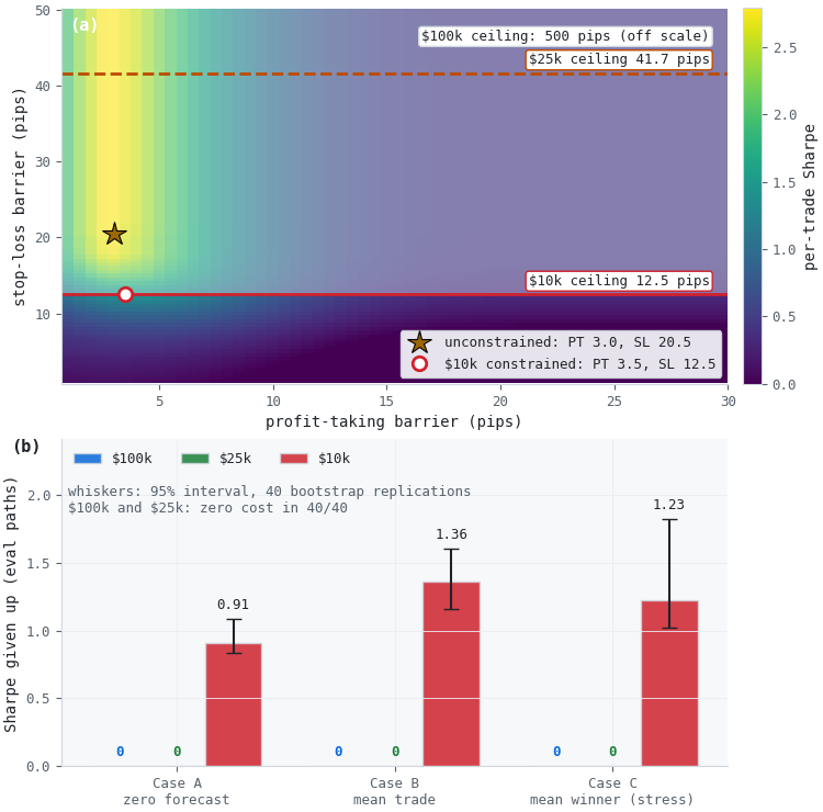
Figure 1. Two-panel illustration of the ceiling against the OTR mesh search on synthetic data

• (a): the simulated Sharpe landscape for Case B, profit-taking against stop-loss in pips. The unconstrained optimum (star) is a 3.0-pip target with a 20.5-pip stop. The $25,000 ceiling (41.7 pips) sits well above it. The $10,000 ceiling (12.5 pips) cuts below it, and the constrained optimum (circle) moves onto the ceiling at a 3.5-pip target and a 12.5-pip stop. The $100,000 ceiling is 500.0 pips and falls entirely off this scale.
• (b): Sharpe given up to the ceiling, by account configuration and forecast case, scored on the evaluation paths. Bars are the full-sample point estimates, and whiskers are 95% intervals over 40 bootstrap replications. The $100,000 and $25,000 configurations give up exactly zero in every replication.

Case	Point estimate	95% interval	Replications binding
A (zero forecast)	0.91	[0.84, 1.08]	40/40
B (mean trade)	1.36	[1.16, 1.61]	40/40
C (stress bound)	1.23	[1.02, 1.83]	40/40

Table 3. Sharpe given up to the $10,000 ceiling, per trade, evaluation paths, 40 bootstrap replications.

The exact zeros in the two slack configurations are a consequence of the mask, not a numerical coincidence. In every replication the unconstrained optimum's stop sat inside both ceilings, so the constrained search returned the identical node. They also serve as a check that the comparison is sound: a constrained search that ever reported a better Sharpe than its own baseline would indicate that the two searches were not evaluating the same set of rules.

What the intervals support is narrower than what the point estimates suggest. The $10,000 configuration binds in all 40 replications and costs between roughly 0.8 and 1.8 Sharpe per trade across the three cases. The intervals for Cases B and C overlap, so the data do not support an ordering between them. Case C's point estimate sitting below Case B's is a sampling outcome, not evidence that a more optimistic forecast makes the ceiling cheaper. These are also per-trade Sharpe ratios on a synthetic process with strong mean reversion (a half-life of about 8.6 bars). They measure the ceiling's cost relative to the rule the process would choose, not a Sharpe any live strategy would earn.

The substantive finding is that the ceiling's relevance is a property of the account configuration, not a universal fact about prop-firm trading. A $100,000 account running two concurrent half-lot positions has a 500.0-pip ceiling against a process whose optimal stop sits between 20 and 23 pips: the constraint is nowhere near binding, and computing it at all is bookkeeping rather than risk management. Shrink the account to $10,000 and raise concurrency to four full lots, and the same process meets a 12.5-pip ceiling that cuts well inside the optimal region. Which regime a given deployment is in has to be checked per configuration; it cannot be assumed from either direction.

The full-strength convention is the conservative one

Table 2 evaluates every ceiling at bet_size=1.0 with positions held independently. That is the right convention for a trader who opens full-size positions and manages each one separately. It is not what PropFirmAwareSizer does. With average_active=True, concurrent signals are averaged into one net position whose size is lot_size times |final_size|, and final_size is rarely close to 1.

Running the sizer chain on synthetic inputs shows how far apart the two conventions can be. The inputs are a fresh Phase 1 $10,000 account, 400 signals with Beta(6, 5) probabilities held in runs of 20 bars, a 60-bar holding period, and step_size=0.05. The sizer emits a nonzero size on 36 of 400 bars, and every one of those sizes equals the 0.05 step. The ceiling must hold for the largest size the sizer emits, here 0.05:

Convention	bet_size	aggregate_exposure	Ceiling (pips)
Full strength, independent	1.00	False	12.5
Full strength, netted	1.00	True	50.0
Largest sizer output, netted	0.05	True	1,000.0

Table 4. The $10,000 ceiling under three exposure conventions, synthetic sizer inputs.

Either relaxation alone lifts the ceiling above the 20.5-pip unconstrained stop. Together they lift it two orders of magnitude past it, and under the sizer as built the $10,000 configuration does not bind either. The inputs in Table 4 are synthetic and chosen to exercise the netting logic; they are not tailored to any strategy. The 0.05 bet size is a property of this setup, in which every nonzero size sits at the minimum step; it is not a general result. The conclusion that survives is methodological: the ceiling must be evaluated at the notional the executor actually sends, and aggregate_exposure must match whether positions are netted or held independently. If live execution holds positions independently, aggregate_exposure=False is correct and the tighter figures in Table 2 apply.

Production Problem: A Ceiling That Doesn't Know What Time of Day It Is

prop_firm_sl_ceiling takes daily_loss_pct as a flat argument. Every other constraint this series has built reads live account state instead: WParamCalibrator calibrates against risk_budget_pct, whatever is left after the day's realized and floating P&L; derisking_factor reads phase_progress as it stands at the moment of the call. When called with rule_set.daily_loss_limit_pct (the standard way to obtain this value), the function always assumes the full daily budget is still available. This remains true whether the session has just started or most of the day's allowance has already been lost.

The gap is not cosmetic. Take the $10,000 configuration from Section 2, with its 12.5-pip ceiling at the start of the day, on the FundedNext Stellar 2-Step rule set. By early afternoon the account has realized a $300 loss, and one of its four positions is still open: one lot, 2 pips (−$20) under water, with its stop 12.5 pips from entry. The rule set is equity-based, so risk_budget_pct nets the floating loss: $320 of the $500 allowance is used, $180 remains, and risk_budget_pct is 1.8%. Passing that figure as daily_loss_pct with four positions gives a 4.5-pip ceiling instead of 12.5.

That substitution is valid only under three conditions, and the function's signature enforces none of them:

• Same denominator: risk_budget_pct is a fraction of state.initial_balance, so account_usd must be that same figure, not the current balance or equity.
• Same accounting basis: risk_budget_pct nets floating P&L only when rule_set.drawdown_basis is "equity", and the ceiling inherits whichever basis is in force.
• Same notion of limit: risk_budget_pct is the smaller of the daily and overall remaining budgets, not the daily allowance alone.

The third condition makes the substitution conservative rather than wrong, but the parameter no longer means what its name says. Even with all three met, the substitution misses one quantity: the risk that open positions still carry. risk_budget_pct subtracts the open position's current floating loss ($20) but not the further $105 it can lose between its current mark and its stop. Dividing by four also treats that open position as a slot still to be filled. live_sl_ceiling reserves the open risk, fixes the denominator to state.initial_balance, and divides what remains across the positions that can still be opened:

def live_sl_ceiling(
    state: PropFirmAccountState,
    open_risk_usd: float,
    n_new: int,
    lot_size: float,
    pip_value_per_lot: float = 10.0,
    bet_size: float = 1.0,
    cost_pips: float = 0.0,
) -> float:
    # docstring omitted: see sizing.py
    if not np.isfinite(open_risk_usd) or open_risk_usd < 0:
        raise ValueError(f"open_risk_usd must be finite and >= 0; got {open_risk_usd!r}")
    budget_usd = state.risk_budget_pct * state.initial_balance - open_risk_usd
    if budget_usd <= 0.0:
        return 0.0
    return prop_firm_sl_ceiling(
        account_usd=state.initial_balance,
        daily_loss_pct=budget_usd / state.initial_balance,
        lot_size=lot_size,
        n_concurrent=n_new,
        pip_value_per_lot=pip_value_per_lot,
        bet_size=bet_size,
        aggregate_exposure=False,
        cost_pips=cost_pips,
    )

Applied to the afternoon state above:

state = PropFirmAccountState(initial_balance=10_000.0, phase=Phase.CHALLENGE_PHASE_1,
                             rule_set=FUNDEDNEXT_STELLAR_2STEP)
state.update(realized_pnl_delta=-300.0, unrealized_pnl=-20.0, fees_and_swaps=0.0)

prop_firm_sl_ceiling(10_000.0, 0.05, 1.0, 4, 10.0)                   # 12.5 pips, start of day
prop_firm_sl_ceiling(10_000.0, state.risk_budget_pct, 1.0, 4, 10.0)  # 4.5 pips
open_risk_usd = (12.5 - 2.0) * 1.0 * 10.0                            # open trade: 10.5 pips to its stop
live_sl_ceiling(state, open_risk_usd, n_new=3, lot_size=1.0)         # 2.5 pips

The static call answers 12.5 pips, the risk_budget_pct substitution 4.5, and the reserved-risk version 2.5. A stop sized from the morning figure is five times wider than what the account can absorb at that point in the day, on the same four-position assumption that made 12.5 pips correct that morning. Passing a 1.0-pip cost_pips reduces the last figure to 1.5 pips, which is already below one σ of this process.

None of this is a defect in the arithmetic: the function computes exactly what it is asked to compute. It is a defect in the calling convention that has grown up around it. daily_loss_pct=rule_set.daily_loss_limit_pct is the obvious argument to reach for, and it is also the one that stops being accurate the moment the account takes its first loss of the day. The fix is at the call site: call live_sl_ceiling each time a fresh ceiling is needed, rather than caching a figure from the start of the session. Nothing about the original function's name or signature signals that the obvious argument is the wrong one.

Edge Case: A Descending Grid

One way to bound an OTR mesh is to replace the stop-loss axis with its own grid, np.linspace(0.5, max_mult, n_nodes), where max_mult is the ceiling divided by σ and n_nodes is the number of stop-loss nodes. That construction assumes max_mult is at least 0.5, the lower bound of the Step 2 example mesh. The assumption holds comfortably for every configuration in Section 5, where the tightest ceiling (12.5 pips) spans 6.26σ. It does not hold universally. A smaller account, more concurrent positions, a larger pip value than the $10 per lot assumed throughout this article, or a more volatile instrument can push the ceiling below half of one bar's σ. When that happens, np.linspace does not raise an error or clamp anything; it returns a decreasing sequence from 0.5 down to max_mult.

max_mult = 0.6 / 1.9982         # 0.6-pip ceiling against sigma = 1.9982 pips
np.linspace(0.5, max_mult, 15)  # 0.500, 0.486, ..., 0.315, 0.300 (sigma units)
# 14 of 15 nodes exceed max_mult: every stop but the last is wider than the ceiling

The consequence is not a harmless reordering. With a 0.6-pip ceiling against σ = 1.9982 pips, every node except the last is wider than the ceiling. A search over that grid is almost entirely a search over infeasible rules, and the Sharpe-maximizing node it reports will very likely be one of them. Nothing in the output flags this: the reported stop simply exceeds the ceiling, reopening the exact breach the ceiling exists to prevent. The obvious guard, moving the lower bound below max_mult, stops the reversal but produces stops far inside one bar's noise. On this article's process, a 0.3σ stop is hit on the first bar by 35% of simulated paths, by the third bar by 55%, and within the 60-bar holding period by 96.5%. A rule that exits on noise that often is not a trading rule.

The fix is structural, and it is the one Section 3 already uses. Define the mesh once and express the ceiling as a mask over its stop-loss nodes. A ceiling below the narrowest node then leaves an empty feasible set, and feasible_sl_mask raises instead of returning a grid. That is the correct outcome, because it states that no rule on this mesh respects the account's limit.

The opinion this leads to is a qualification of Step 5c rather than a disagreement with it. The book treats a manager-imposed stop as an input to the search. In a prop-firm account it is also a feasibility test. A configuration whose ceiling sits below half of one bar's σ is saying that the position size is wrong for the account, and no choice of barriers repairs that. The search should fail loudly in that case, so that the decision goes back to sizing, where it belongs.

Conclusion

Key takeaways:

• A hard ceiling constrains one axis of the search, and only one. Following AFML Step 5c, the profit-taking barrier is still searched over its full range; the ceiling excludes stop-loss nodes only.
• Build the constrained search as a subset of the unconstrained mesh. Two independent np.linspace grids do not share nodes, so a regridded search can beat its own baseline; a mask over one shared mesh cannot.
• Whether the ceiling costs anything has to be checked, not assumed. At the full-strength convention it bound in one of three configurations, in all 40 bootstrap replications, at a cost of 0.91 (95% interval 0.84 to 1.08) to 1.36 (1.16 to 1.61) Sharpe per trade for Cases A and B. The other two configurations gave up exactly zero.
• Evaluate the ceiling at the notional actually executed. On synthetic sizer inputs with netting, the same $10,000 ceiling rose from 12.5 to 1,000.0 pips and did not bind at all.
• Fit the O-U to within-trade paths, not to a sequence of trade outcomes. Pairing consecutive trades returns a σ equal to the dispersion of outcomes rather than the per-bar innovation, which makes the ceiling look more binding than it is.
• The ceiling is a nominal bound. Execution costs can be subtracted through cost_pips; gaps through the stop cannot be bounded by any stop distance.
• A static constraint next to dynamic ones needs a live counterpart. Substituting risk_budget_pct requires a shared denominator and accounting basis, and it still misses the risk carried by open positions; live_sl_ceiling reserves it.
• An implicit range assumption is still an assumption once its inputs change. A reversed np.linspace grid tests stops wider than the ceiling; a mask over a fixed mesh raises instead.

Four parts in, the constraint chain this series set out to build has all of its pieces: a configurable rule set, an account state that tracks it across days and calls, three sizing modifiers reading three distinct facts about the account, and a stop-loss ceiling bounding the one search in this pipeline that was never account-state-aware to begin with. What remains is validating the whole chain together against real historical data rather than one modifier at a time. That is the natural next step, not yet scoped.

Attached Files

	File	Module	Description
1.	__init__.py	afml	Package marker for the afml namespace.
2.	__init__.py	afml.prop_firm	Package exports, including live_sl_ceiling.
3.	phase.py	afml.prop_firm	Phase enumeration shared by the rule set and the account state.
4.	rule_set.py	afml.prop_firm	PropFirmRuleSet and FUNDEDNEXT_STELLAR_2STEP, the rule set used in Section 6.
5.	account_state.py	afml.prop_firm	PropFirmAccountState, the source of risk_budget_pct.
6.	sizing.py	afml.prop_firm	prop_firm_sl_ceiling with input validation and cost_pips, live_sl_ceiling, and PropFirmAwareSizer, used for Table 4.
7.	__init__.py	afml.bet_sizing	Package exports required by the imports in sizing.py.
8.	bet_sizing.py	afml.bet_sizing	bet_size_probability, the first stage of PropFirmAwareSizer.
9.	ch10_snippets.py	afml.bet_sizing	AFML Chapter 10 snippets (get_w, bet_size_sigmoid) used by the sizer.
10.	ef3m.py	afml.bet_sizing	EF3M mixture fitting. Not used in this article; required because bet_sizing.py imports it.
11.	otr_ceiling_sim.py		Synthetic O-U simulation, shared-mesh constrained and unconstrained search, and bootstrap intervals. Reproduces Tables 1 to 4.
12.	otr_ceiling_figure.py		Draws Figure 1 from the results file written by otr_ceiling_sim.py.
13.	test_otr_ceiling.py		Tests for input validation, the live ceiling, the estimators, and the subset property of the constrained search.
14.	ERRATA_ou_estimation.md		Full rationale for the eq. (13.6) estimator correction, the mesh comparison fixes, and a checklist for future O-U work.

Place all files under MQL5/Files/afml/, keeping the prop_firm and bet_sizing subfolders, and run the scripts from MQL5/Files: python afml/otr_ceiling_sim.py, then python afml/otr_ceiling_figure.py, and python -m pytest afml/test_otr_ceiling.py -q for the tests. The code requires NumPy, pandas, SciPy, Numba, Matplotlib, Pillow, and pytest.

Further Reading

• López de Prado, M. (2018). Advances in Financial Machine Learning, Chapter 13. John Wiley & Sons.
• Bailey, D. H., and López de Prado, M. (2012). The Sharpe ratio efficient frontier. Journal of Risk, 15(2), 3–44.