Hyperdimensional Computing: Learning in One Integer Add, and the Nulls That Judge It

Contents

• Introduction
• What the library does, before any theory
• Why the dimension is the whole idea
• Bind, bundle and permute
• The codebook: names, and quantities
• Encoding a bar, and a window of bars
• Learning is integer addition
• The facade: a purged split, and a free update
• A reference that is not an approximation
• What real markets say
• The indicator
• Cost
• Conclusion

Introduction

Most machine learning methods that reach MetaTrader arrive with some version of the same bill attached. Training is expensive, so you retrain on a cadence and hope nothing important happened in between. The model is a block of floating point weights, so reproducing a result on another machine means reproducing a sequence of floating point operations in the same order. And when the model finally prints a number, you have no idea what that number would look like if the model knew nothing at all.

Hyperdimensional Computing, set out by Pentti Kanerva in 2009 and also known as Vector Symbolic Architecture, addresses all three at once, by giving up something most would not think they could: no single weight in the model means anything. Every concept, feature name and quantity is one very long random vector, and there are exactly three operations. Bind is XOR, bundle is an element-wise majority, permute is a cyclic shift. That is the whole algebra.

What you get in exchange is worth having in a trading terminal specifically. Learning is an integer add into an accumulator, so a model absorbs one more labeled row in a few hundred microseconds rather than waiting for a refit. The classifier core is integer and bitwise end to end, so a reference implementation of that core does not produce a similar model, it produces the same model. And because two unrelated hypervectors have a known distance distribution, the noise floor a reading is measured against is a closed-form expression rather than a permutation run that costs seconds per bar.

Each of those three has a boundary, and this article marks the boundary where it arises. A row carries a label that reads five bars ahead, so the newest row that can be folded in sits five bars behind the close. Feature engineering upstream of the encoder is ordinary double arithmetic, and only what happens from the quantizer onwards is exact. And the closed-form band describes unrelated prototypes, which the prototypes of a trained model are not.

This article builds that library. Nothing of the kind exists in the MQL5 catalog, so every part is from scratch: the algebra, the codebook, the classifier, and the tests that judge them. It is written for a developer who wants a classifier they can reason about completely, and it is honest about what the finished library finds in price data, which is very little. The last two sections are about measuring that, because a method that cannot be refuted is not a method.

What the library does, before any theory

The finished library builds a two-class model from six causal features on a bar, and reports a signed decision variable called the margin. Here is what its market scan prints on XAUUSDm D1 over 3000 bars, comparing a model kept up to date one bar at a time against the same model refitted from scratch on a cadence:

=== 7. online updating against a batch refit ===
      670 rows scored: online 0.4866, batch-refit 0.5060, they agree 38.1%
      cost: 670 online updates 226 ms total (337 us each), 27 batch refits 9571 ms total
=== 8. cost ===
      one full fit over 1674 rows: 425 ms (min of 3)
      which is 254 us per row, and the encoding is nearly all of it

The cost line is worth reading twice. Six hundred and seventy online updates took 226 milliseconds, so one update costs about 337 microseconds. Twenty-seven full refits over the same span took 9.6 seconds, so one refit of that span costs about 354 milliseconds. They differ by three orders of magnitude, but they are not the same unit of work: the update folds in one row, the refit re-encodes the whole span. Per row the full fit costs 254 microseconds against the update's 337, so nothing here says the accumulator is a faster way to encode a row. What it buys is that the history never has to be encoded again. Nor is the gap bought with an approximation: with the perceptron corrections switched off, so the comparison isolates the accumulator, the test suite asserts that folding one row in incrementally reproduces the full refit to the bit, worst error 0 bits. The accuracy figures above are a separate question, and the section on the facade answers it.

The scan also reports what the model is worth as a predictor, which is nothing. Its hold-out edge over the majority class is negative, negative in all six walk-forward folds, and comfortably inside two separate nulls. Both results matter and neither cancels the other.

Why the dimension is the whole idea

Start with the property everything else rests on. Take two random vectors of D bits and count the positions where they differ. That count is Binomial(D, 1/2), so it has mean D/2 and standard deviation sqrt(D)/2. Now express it as a similarity in the range from minus one to one:

sim = 1 - 2 * hamming / D

The mean becomes 0 and the standard deviation becomes 1 / sqrt(D). At D = 256 that is 0.0625, loose enough that about one unrelated pair in twenty looks more than 12 percent alike. At D = 4096 it is 0.0156. Only the dimension changed, and the consequence is that unrelated concepts stop colliding. Figure 1 draws the distribution at three dimensions using the library's own generator.

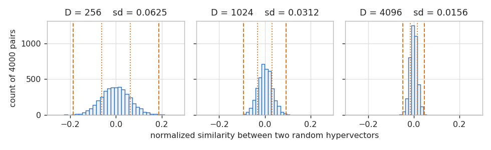
Fig. 1. The same experiment at three dimensions. The dotted lines mark one standard deviation and the dashed lines three. The distribution does not change shape, it only narrows, and that narrowing is what lets many facts share one vector

The library measures this rather than assuming it. On 400 pairs at D = 2048 the mean distance comes out 1025.54 against a predicted 1024.0, and the standard deviation 22.15 against a predicted 22.63. That is the whole justification for a noise band, and why it costs nothing to draw.

Because the distance is the only measurement the algebra makes, it is kept as an integer everywhere and converted to a float only for display. The features that feed the algebra are a separate matter and they are doubles; the exactness begins at the quantizer. The primitive is a straight population count over the XOR:

//+------------------------------------------------------------------+
//| Integer bit distance: the primitive every similarity is built on |
//|                                                                  |
//|  SWAR and not the table: over three runs at D=2048, SWAR 0.057   |
//|  to 0.229 us against the table's 0.117 to 0.398. The 64 KB       |
//|  table misses L1, and it is kept as the independent check.       |
//+------------------------------------------------------------------+
int CHDCVector::Hamming(const ulong &a[], const ulong &b[]) const
  {
   int total = 0;
   for(int i = 0; i < m_w; i++)
      total += HDCPopSwar(a[i] ^ b[i]);
   return(total);
  }

The SWAR trick in HDCPopSwar adds bits in parallel inside a 64-bit register. A 65536-entry lookup table is also in the file, faster on paper and slower in practice because 64 KB does not stay in L1. It stays as an independent check on the SWAR version, and the test asserts the two agree on 5000 random words.

One constraint is worth stating plainly because it is enforced in code. D must be a multiple of 64. A ragged final word carries unused bits, and a population count cannot know they are not data, so every similarity would be wrong by an amount that depends on the seed. CHDCVector::Init refuses any other dimension, and the test checks that 1000 is refused and 1024 accepted.

Bind, bundle and permute

Three operations, each with one job. Bind associates two things and produces something unrelated to both. It is XOR, it is its own inverse, and it preserves every distance, which is the property that makes the rest of the algebra work:

//+------------------------------------------------------------------+
//| bind: XOR. Self inverse, and it preserves every distance         |
//+------------------------------------------------------------------+
void CHDCVector::Bind(const ulong &a[], const ulong &b[], ulong &out[]) const
  {
   Alloc(out);
   for(int i = 0; i < m_w; i++)
      out[i] = a[i] ^ b[i];
  }

//+------------------------------------------------------------------+
//| bind in place, for accumulating a chain                          |
//+------------------------------------------------------------------+
void CHDCVector::BindInto(const ulong &a[], ulong &acc[]) const
  {
   for(int i = 0; i < m_w; i++)
      acc[i] = acc[i] ^ a[i];
  }

Because XOR is an isometry, binding a whole set of vectors with the same key moves them all without changing any distance between them. That is how a role attaches to a value without destroying the grading between neighboring values, and it is why the encoder can bind first and bundle afterwards.

Permute is a cyclic rotation of the entire D-bit string. Rotating a hypervector produces something unrelated to the original, which is exactly what is wanted: it is how position in a sequence is marked, so that the same three bars in a different order become a different vector.

//+------------------------------------------------------------------+
//| permute: rotate the whole D-bit string left by shift             |
//|                                                                  |
//|  Word level, so it costs W steps and not D. Because D is a       |
//|  multiple of 64 this is an exact rotation with no ragged edge.   |
//+------------------------------------------------------------------+
void CHDCVector::Permute(const ulong &a[], const int shift, ulong &out[]) const
  {
   Zero(out);
   int s = shift % m_d;
   if(s < 0)
      s += m_d;

   int ws = s / 64;
   int bs = s % 64;

   for(int i = 0; i < m_w; i++)
     {
      ulong lo = (bs == 0 ? a[i] : (a[i] << bs));
      out[(i + ws) % m_w] |= lo;
      if(bs != 0)
        {
         ulong hi = a[i] >> (64 - bs);
         out[(i + ws + 1) % m_w] |= hi;
        }
     }
  }

Note that the rotation is over the bit string and not the word array, which is why the code carries bits across word boundaries. The test asserts that permuting and then unpermuting is the identity to 0 bits.

Bundle is the superposition operator, and it is the only one that is not exactly invertible. It takes an element-wise majority: for each of the D bit positions, count how many inputs have a one there and take whichever wins. The result is similar to every input and unrelated to everything else, and the implementation goes through a signed accumulator so that weights are possible:

//+------------------------------------------------------------------+
//| Add a hypervector into an integer accumulator as +1 / -1         |
//+------------------------------------------------------------------+
void CHDCVector::AddSigned(const ulong &v[], const int weight, int &acc[]) const
  {
   if(ArraySize(acc) < m_d)
      ArrayResize(acc, m_d);

   int at = 0;
   for(int i = 0; i < m_w; i++)
     {
      ulong word = v[i];
      for(int b = 0; b < 64; b++, at++)
        {
         acc[at] += ((word & 1) != 0 ? -weight : weight);
         word >>= 1;
        }
     }
  }

//+------------------------------------------------------------------+
//| Threshold an accumulator back to packed bits                     |
//|                                                                  |
//|  Positive means bit 0. An exact zero has no majority and takes   |
//|  its bit from the tie vector, so even-sized bundles do not all   |
//|  resolve the same way and correlate with each other.             |
//+------------------------------------------------------------------+
void CHDCVector::PackSign(const int &acc[], const ulong &tie[], ulong &out[]) const
  {
   Zero(out);
   bool haveTie = (ArraySize(tie) == m_w);

   for(int i = 0; i < m_d; i++)
     {
      int v = acc[i];
      bool one = (v < 0);
      if(v == 0 && haveTie)
         one = (((tie[i >> 6] >> (i & 63)) & 1) != 0);
      if(one)
         out[i >> 6] |= ((ulong)1 << (i & 63));
     }
  }

The tie vector is what keeps that correlation from being systematic, and because it is drawn from the same seeded stream as everything else, the coin flip it stands in for is stable across runs and across languages. Figure 2 measures what each operation does.

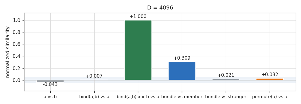
Fig. 2. Every bar is one measurement at D = 4096, and the shaded strip is three standard deviations of the noise floor. Only two comparisons leave it: unbinding recovers the input exactly, and a bundle stays visibly close to its own members

A bundle cannot hold unlimited things, and the limit is a closed form rather than a rule of thumb: the expected similarity between a bundle and one of its own members is a central binomial term, which the library evaluates as a product of small ratios so nothing overflows.

//+------------------------------------------------------------------+
//| Expected similarity between a majority bundle of k and a member  |
//|                                                                  |
//|  Exactly C(m,m/2)/2^m with m = k-1 for odd k and m = k for even  |
//|  k, which the tie vector pads to odd. Evaluated as the product   |
//|  of (2i-1)/(2i) so nothing overflows.                            |
//+------------------------------------------------------------------+
double HDCBundleSimilarity(const int k)
  {
   if(k <= 0)
      return(0.0);
   if(k == 1)
      return(1.0);

   int m = ((k % 2) == 1 ? k - 1 : k);
   int n = m / 2;

   double p = 1.0;
   for(int i = 1; i <= n; i++)
      p *= (double)(2 * i - 1) / (double)(2 * i);
   return(p);
  }

That closed form is only half the answer. What a caller wants is not the similarity but whether a member can still be picked out of a codebook, and that depends on the competition. The nearest of n unrelated distractors sits about sqrt(2 ln n) standard deviations from the mean, which for a 256-entry codebook is 3.33, so recall should hold while the member's signal clears 3.33 sd and break shortly after. Measured at D = 2048, recall is a perfect 1.000 down to 6.5 sd, 0.974 at 4.6 sd, and 0.814 at 3.2 sd. The theory said where it would break and it broke there.

That result bounds one component rather than describing the finished model. It is a statement about a plain majority bundle probed against a codebook, and the classifier does something else: it bundles six bound levels per bar, accumulates weighted rows into two classes, thresholds the result and then corrects it with perceptron passes. The capacity curve tells you when a bundle stops being readable. It does not predict the accuracy of the model built on top of it.

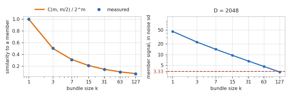
Fig. 3. The left panel is the closed form with measurements on top of it. The right panel converts the same curve into standard deviations, and the dashed line at 3.33 is where the nearest of 256 distractors sits, so recall breaks where the blue curve reaches it

The codebook: names, and quantities

Everything in the algebra is a random vector, but a feature value cannot be. Two names such as "ret1" and "maDist" have no order, so independent random vectors suit them. A quantity is different: a bar whose one-bar return sits at 1.9 standard deviations and a bar at 2.0 must come out similar, or the encoding throws away the structure it exists to capture.

The answer is a level ladder. Level 0 is a random vector, and each step up flips a fresh slice of one shared random permutation of the bit positions, the slices disjoint. Because they are disjoint, the bits separating level i from level j are exactly the bits flipped between them, so the distance between any two levels equals the difference of their cuts, with no approximation. Spend D/2 flips across the ladder and the extremes land exactly orthogonal.

//+------------------------------------------------------------------+
//| Build a level ladder, or return the one already held             |
//+------------------------------------------------------------------+
int CHDCMemory::MakeLevels(const string name, const int count)
  {
   int at = FindLadder(name);
   if(at >= 0)
      return(at);
   if(count < 2)
      return(-1);

   at = m_ladCount;
   int base = (at == 0 ? 0 : m_ladOffset[at - 1] + m_ladLevels[at - 1] * m_w);

   ArrayResize(m_ladName, at + 1);
   ArrayResize(m_ladLevels, at + 1);
   ArrayResize(m_ladOffset, at + 1);
   ArrayResize(m_ladBits, base + count * m_w);

   m_ladName[at]   = name;
   m_ladLevels[at] = count;
   m_ladOffset[at] = base;

   //--- level 0 is random
   ulong cur[];
   m_v.Random(m_rng, cur);
   for(int w = 0; w < m_w; w++)
      m_ladBits[base + w] = cur[w];

   //--- one shared permutation, Fisher-Yates walking downwards
   int perm[];
   ArrayResize(perm, m_d);
   for(int i = 0; i < m_d; i++)
      perm[i] = i;
   for(int i = m_d - 1; i > 0; i--)
     {
      int j = m_rng.Below(i + 1);
      int t = perm[i];
      perm[i] = perm[j];
      perm[j] = t;
     }

   //--- each step flips the next disjoint slice
   for(int k = 1; k < count; k++)
     {
      int lo = HDCLevelCut(k - 1, m_d, count);
      int hi = HDCLevelCut(k, m_d, count);
      for(int t = lo; t < hi; t++)
         m_v.FlipBit(cur, perm[t]);
      for(int w = 0; w < m_w; w++)
         m_ladBits[base + k * m_w + w] = cur[w];
     }

   m_ladCount = at + 1;
   return(at);
  }

The cut function is one line of integer arithmetic, cut(k) = k * (D/2) / (levels - 1), and it is shared with the reference implementation so that both sides place their flips identically. Figure 4 shows the result: not close to the closed form, equal to it.

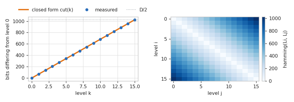
Fig. 4. Sixteen levels at D = 2048. The measured points sit on the closed form rather than near it, and the matrix on the right is the same statement for every pair at once

The test suite checks all 256 pairs of a 16-level ladder and reports a worst error of 0 bits, with the extremes at 1024 of 2048. That exactness is not decoration: it means a ladder can be regenerated anywhere from a seed and a count, which is what makes the cross-check an equality.

One thing about the codebook is easy to break by accident: registration order is part of the contract. Symbols and ladders are drawn from a single stream, so the order in which they are requested decides which bits each one gets. The facade and the reference implementation register the same names in the same sequence; change the order on one side only and every vector in the codebook changes.

Encoding a bar, and a window of bars

Six features per bar, all causal and all scale free. Scale free matters because a level ladder quantizes against a fixed range, and a raw price range on gold has nothing to do with one on EURUSD:

      int at = m_rows * HDC_NFEAT;
      m_x[at + 0] = ret[i] / sd;
      m_x[at + 1] = ret5 / (sd * MathSqrt(5.0));
      m_x[at + 2] = (r[i].close - r[i].open) / range;
      m_x[at + 3] = range / atr;
      m_x[at + 4] = (upper - lower) / range;
      m_x[at + 5] = (r[i].close - ma) / maDen;

Each is a ratio that a change of instrument leaves alone, so one ladder quantizes gold and EURUSD alike. Nothing is standardized across the whole sample, because a feature standardized with statistics drawn from the entire history has seen the future.

The label uses the same discipline in the other direction:

      //--- the label looks forward only, and only when one was asked for
      int y = -1;
      if(withTarget)
        {
         double fwd = 0.0;
         for(int k = i + 1; k <= i + m_horizon; k++)
            fwd += ret[k];
         double bar2 = m_threshK * sd * MathSqrt((double)m_horizon);
         if(MathAbs(fwd) < bar2)
           {
            m_flatDropped++;
            continue;
           }
         y = (fwd > 0.0 ? HDC_UP : HDC_DOWN);
        }

A row is labeled UP or DOWN by the sign of the forward return over the horizon, but only when that move clears k * sd * sqrt(horizon). The sd * sqrt(horizon) part is the move a random walk of that length would typically produce, and k scales it: the shipped value is 0.5, so a row has to travel half of a typical walk before it earns a label. Rows that do not clear it are dropped rather than assigned to a third class, which on the gold sample removes 1199 of 2873 candidate rows and leaves 1674. Dropping them is deliberate: a model that has to separate the flat middle spends all its capacity there.

It is also a choice with a cost, because the filter reads the future. Whether a bar clears the threshold is decided by the five bars after it, so the rows the model trains and is scored on are a subsample selected with information that does not exist when the bar closes. Live, the question the filter asks cannot be asked. Everything measured later is therefore measured on a conditional subsample: given that a bar did not stay inside the flat band, how well is its direction classified. That is a legitimate question, and not the same question as how well the model would do pointed at every bar.

The library offers no abstain rule to close that gap, and it should be clear that the margin band is not one. The section on the band shows why: for a fitted model the band is not a significance test, and a two-class model with the flat rows removed always answers UP or DOWN. A causally available rule for when not to act is left to the caller, and it is the first thing anyone building on this would have to add.

Now the encoding. A bar becomes a record: each feature is quantized to a level, the level is bound with that feature's role vector, and the six results are bundled. Binding first stops the six from being confused with each other; bundling second keeps the record graded, so a bar that is a little different produces a record that is a little different. A window of bars becomes a sequence: each record is rotated by its distance from the newest bar and all of them are XORed together.

//+------------------------------------------------------------------+
//| One bar's feature values to a record hypervector                 |
//+------------------------------------------------------------------+
void CHDCEncoder::Record(const double &values[], ulong &out[])
  {
   ulong flat[];
   ArrayResize(flat, m_nRole * m_w);

   ulong role[], lvl[], bound[];
   for(int f = 0; f < m_nRole; f++)
     {
      m_mem.GetSymbol(m_roleId[f], role);
      m_mem.GetLevel(m_ladId[f], Quantize(f, values[f]), lvl);
      m_v.Bind(role, lvl, bound);
      for(int w = 0; w < m_w; w++)
         flat[f * m_w + w] = bound[w];
     }

   ulong tie[];
   TieVector(tie);
   m_v.Bundle(flat, m_nRole, tie, out);
  }

//+------------------------------------------------------------------+
//| Bind count permuted records into one sequence hypervector        |
//|                                                                  |
//|  records is flat and records[0] is the OLDEST, which is the      |
//|  position that carries the largest shift.                        |
//+------------------------------------------------------------------+
void CHDCEncoder::Sequence(const ulong &records[], const int count, ulong &out[])
  {
   m_v.Zero(out);
   if(count <= 0)
      return;

   ulong one[], shifted[];
   m_v.Alloc(one);
   for(int i = 0; i < count; i++)
     {
      for(int w = 0; w < m_w; w++)
         one[w] = records[i * m_w + w];
      m_v.Permute(one, count - 1 - i, shifted);
      m_v.BindInto(shifted, out);
     }
  }

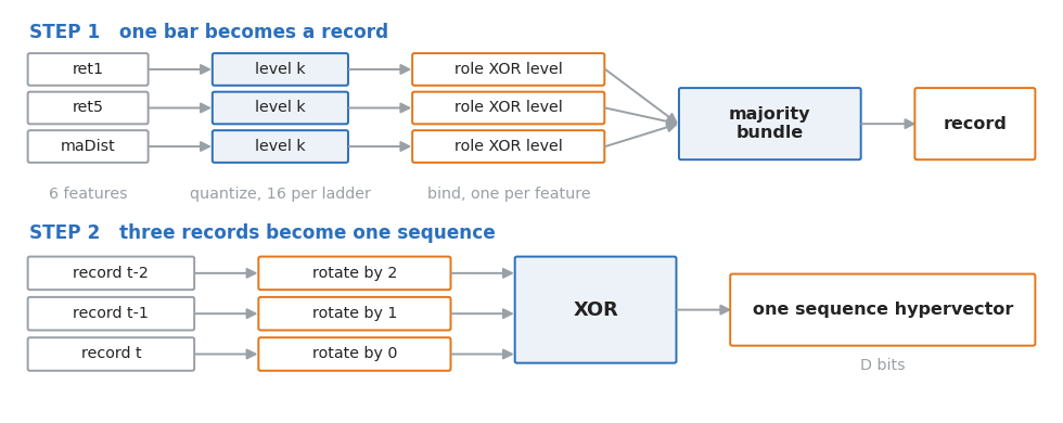
Fig. 5. The encoding, end to end. Bind separates the roles, bundle keeps the record graded, and the rotation before the final XOR is the only thing that makes order matter

The rotation is what turns a bag of bars into a sequence, and the test measures it rather than asserting a threshold. Reversing three bars moves the sequence by 1658 bits of 4096, while changing one bar in the middle moves it by 424. The claim checked is the relative one, because the heuristic that unrelated vectors sit near D/2 apart belongs to random vectors, and a record is a bundle of bound levels.

One detail in SetRangesFrom is worth calling out. Quantizer bounds are taken from training rows only, and both tails are trimmed by two percent before the range is set. Without the trim, one outlier bar sets the range and every ordinary bar lands in the same level, producing a codebook that is technically correct and completely uninformative.

That completes the encoder, so this is the point to put the shipped settings in one place. Every number in this article was produced at D = 4096 bits, 16 levels per ladder, a 3-bar sequence, a 5-bar label horizon at k = 0.5, a 100-bar trailing volatility window, 2 perceptron passes, and 30 percent of the training range held out. Each is an input on both the market scan and the indicator, so none is baked in.

Learning is integer addition

A class is represented by one accumulator of D signed integers. To learn an example, walk its bits and add plus one where the bit is zero and minus one where it is one. To turn the accumulator into something the algebra can measure, threshold it back to D bits:

//+------------------------------------------------------------------+
//| Add one example into a class accumulator                         |
//|                                                                  |
//|  A negative weight subtracts, which is what a perceptron         |
//|  correction does, so Seen tracks the net weight in each class.   |
//+------------------------------------------------------------------+
void CHDCClassifier::Add(const ulong &hv[], const int cls, const int weight = 1)
  {
   if(cls < 0 || cls >= m_n)
      return;

   int at = cls * m_d;
   int pos = 0;
   for(int i = 0; i < m_w; i++)
     {
      ulong word = hv[i];
      for(int b = 0; b < 64; b++, pos++)
        {
         m_acc[at + pos] += ((word & 1) != 0 ? -weight : weight);
         word >>= 1;
        }
     }
   m_seen[cls] += weight;
  }

//+------------------------------------------------------------------+
//| Threshold every accumulator into its query-time prototype        |
//+------------------------------------------------------------------+
void CHDCClassifier::Finalize(void)
  {
   int  col[];
   ulong packed[];
   ArrayResize(col, m_d);

   for(int c = 0; c < m_n; c++)
     {
      for(int i = 0; i < m_d; i++)
         col[i] = m_acc[c * m_d + i];
      if(m_haveTie)
         m_v.PackSign(col, m_tie, packed);
      else
        {
         ulong none[];
         m_v.PackSign(col, none, packed);
        }
      for(int w = 0; w < m_w; w++)
         m_proto[c * m_w + w] = packed[w];
     }
  }

The distinction between the accumulator and a bundle is easy to miss, and worth stating precisely because the obvious reading of it is wrong. A majority bundle saturates: at 63 members its similarity to any one of them is about 0.10, and by 501 it is 1.3 standard deviations above noise, barely visible. The accumulator does not escape that. Thresholded with every example weighted one it is the majority bundle, bit for bit, with the same ceiling. What it keeps that a bundle throws away is the weights. Measured at 501 examples: add one ten times rather than once and the prototype recovers it at a similarity of 0.3242, where a plain majority bundle of the same 501 gives 0.0283. The cause of that gap is the weight and not the accumulator, which is how the library's own test states it. The accumulator is what makes a weight expressible at all, which is what the perceptron corrections need. The sum is held in int, so its range is finite rather than unbounded: at weight one it would take on the order of two billion examples to matter, but it is a bound and not the absence of one. Only the query-time prototype is thresholded, and it is rebuilt whenever the model changes.

Training is then one pass of adds, followed by perceptron corrections:

//+------------------------------------------------------------------+
//| One pass, then up to passes perceptron corrections               |
//|                                                                  |
//|  samples is flat, count consecutive hypervectors. Stops early    |
//|  once a pass changes nothing.                                    |
//+------------------------------------------------------------------+
int CHDCClassifier::Fit(const ulong &samples[], const int &labels[],
                        const int count, const int passes)
  {
   Reset();
   ulong one[];
   m_v.Alloc(one);

   for(int i = 0; i < count; i++)
     {
      for(int w = 0; w < m_w; w++)
         one[w] = samples[i * m_w + w];
      Add(one, labels[i], 1);
     }
   Finalize();

   int done = 0;
   for(int p = 0; p < passes; p++)
     {
      int changed = 0;
      for(int i = 0; i < count; i++)
        {
         for(int w = 0; w < m_w; w++)
            one[w] = samples[i * m_w + w];
         int pred = Predict(one);
         if(pred != labels[i])
           {
            Add(one, labels[i], 1);
            Add(one, pred, -1);
            changed++;
           }
        }
      Finalize();
      done++;
      m_lastChanged = changed;
      if(changed == 0)
         break;
     }
   m_lastPasses = done;
   return(done);
  }

The correction is the classical one: when a training row is predicted wrongly, add it to the class it should have gone to and subtract it from the class that won. There is no learning rate, no gradient and no floating point anywhere in this function. The loop stops early when a pass changes nothing, and LastPasses and LastChanged let a caller tell a converged fit from one that ran out of passes.

The decision variable is the difference of the two distances, and it too is an integer:

marginBits = hamming(x, prototype_DOWN) - hamming(x, prototype_UP)

Positive means the row sits closer to the UP prototype. Normalizing by 2/D puts it on the same scale as a similarity, and because two near-independent distances are subtracted the variance adds: the standard deviation of a margin between two prototypes that know nothing is sqrt(2/D), which at D = 4096 is 0.02210. The test builds two prototypes from single random vectors, probes them 800 times, and measures 0.02151, with 4 of 800 probes outside a three standard deviation band.

The facade: a purged split, and a free update

The facade owns the codebook, the encoder and the classifier, and exists mainly to make two things hard to get wrong. The first is the validation split. Rows here are overlapping windows: two adjacent rows share bars, and their labels share forward returns. Cut the sample in the middle and the rows either side are almost the same rows, so a hold-out built that way is not out of sample at all. The fix is a purge gap:

   //--- purge, then split oldest-for-training newest-for-validation
   int purge = m_ngram + data.Horizon();
   int valN  = (int)MathFloor(valPct * 0.01 * n);
   if(valN < 0)
      valN = 0;
   if(valN > 0 && n - valN - purge < 40)
      valN = 0;

   int trainHi = (valN > 0 ? hi - valN - purge : hi);
   int valLo   = hi - valN + 1;

   //--- the quantizer sees the TRAINING rows and nothing else, so the
   //    held-out rows do not reach the model through the bin edges
   m_matRows = -1;                                 // the dataset may have changed
   SyncMatrix(data);
   int trainSpan = trainHi - lo + 1;
   double sub[];
   ArrayResize(sub, trainSpan * HDC_NFEAT);
   for(int r = 0; r < trainSpan; r++)
      for(int f = 0; f < HDC_NFEAT; f++)
         sub[r * HDC_NFEAT + f] = m_mat[(lo + r) * HDC_NFEAT + f];
   m_enc.SetRangesFrom(sub, trainSpan, 2.0);

The gap is ngram + horizon rows wide, which is the span over which two rows share raw bars or share forward returns, and it is eight rows at the shipped settings. The split is also ordered rather than random: the older rows train and the newest rows validate, because a random split lets the model learn from bars that come after the ones it is tested on.

Note the order of those two blocks, because it is easy to get backwards. The split is decided first, and only then are the quantizer bounds computed, from trainSpan rows rather than the whole range. A bin edge summarizes a distribution, so setting it from rows the model is about to be tested on lets the hold-out reach the model sideways, without a single label crossing the gap. The cross-check recomputes those bounds from the training rows alone and demands the same numbers.

That gap is not the full extent of the dependence between the two sides. Four of the six features are trailing estimates: a 100-bar standard deviation, a 14-bar ATR, a 20-bar average. Two rows a hundred bars apart are computed from overlapping windows of the same bars, so their features stay correlated long after their bars and their labels have stopped overlapping. Widening the gap to cover that would cost a hundred rows of a 1674-row sample and would still leave the correlation, because the windows are nested rather than adjacent. So the gap removes the sharing a naive cut creates in the bars and in the labels, and the features keep a slower dependence that no gap of this shape removes. The hold-out numbers later should be read with that in mind.

The second thing is the online update, and it is the reason to build this library rather than a different one:

//+------------------------------------------------------------------+
//| Fold one more labeled row into the model, no refit               |
//|                                                                  |
//|  An update is an integer add into the accumulators, so a live    |
//|  model can move on every closed bar without any refit.           |
//+------------------------------------------------------------------+
bool CHDC::Update(CHDCData &data, const int row)
  {
   if(!m_ready || !data.HasTarget())
      return(false);
   int y = data.Y(row);
   if(y < 0)
      return(false);

   ulong hv[];
   EncodeAt(data, row, hv);
   m_clf.Add(hv, y, 1);
   m_clf.Finalize();
   return(true);
  }

Encode the row, add it into one accumulator, rebuild the prototypes. No re-encoding of history and no optimizer state. The test asserts that a model trained on n rows and a model trained on n minus one rows with the last folded in afterwards produce prototypes that agree to 0 bits. That comparison runs with the perceptron passes switched off, which is the point rather than a weakness: what it isolates is the accumulator, and an integer sum does not care in which order its terms arrived.

Switch the corrections back on and the two paths part company, which is worth stating because the natural assumption is the opposite. Plain adds carry weight one, while the perceptron corrections in a batch fit accumulate larger weights, so as online adds pile up they gradually dilute those corrections. Measured over 670 rows on gold, the online arm scored 0.4866, the refitted arm 0.5060, and the two agreed on only 38.1 percent of rows. Neither is broken: they are different models, and a caller choosing between them should know that.

A reference that is not an approximation

Cross-checking a numerical library against another implementation usually means agreeing to some tolerance, and the tolerance is a judgment call. Here it is not, because there is no floating point in the pipeline. Bind is XOR, bundle is an integer majority, similarity is a population count, and learning is an integer add. The only float in the library is the final division by D for display.

The generator is shared as well. MQL5's ulong wraps exactly like a masked Python integer, so splitmix64 feeding xorshift64* produces identical 64-bit words in both implementations:

//+------------------------------------------------------------------+
//| splitmix64 once, so any seed becomes a usable state              |
//+------------------------------------------------------------------+
void CHDCRandom::Seed(const ulong seed)
  {
   ulong z = seed + 0x9E3779B97F4A7C15;
   z = (z ^ (z >> 30)) * 0xBF58476D1CE4E5B9;
   z = (z ^ (z >> 27)) * 0x94D049BB133111EB;
   z = z ^ (z >> 31);
   m_state = (z != 0 ? z : 0x9E3779B97F4A7C15);   // zero is xorshift's fixed point
  }

//+------------------------------------------------------------------+
//| One xorshift64* draw                                             |
//+------------------------------------------------------------------+
ulong CHDCRandom::NextU64(void)
  {
   ulong s = m_state;
   s ^= s >> 12;
   s ^= s << 25;
   s ^= s >> 27;
   m_state = s;
   return(s * 0x2545F4914F6CDD1D);
  }

And the same two steps in the Python reference:

    def seed(self, s):
        z = (s + 0x9E3779B97F4A7C15) & MASK64
        z = ((z ^ (z >> 30)) * 0xBF58476D1CE4E5B9) & MASK64
        z = ((z ^ (z >> 27)) * 0x94D049BB133111EB) & MASK64
        z = z ^ (z >> 31)
        self.state = z if z != 0 else 0x9E3779B97F4A7C15

    def next_u64(self):
        s = self.state
        s ^= s >> 12
        s = (s ^ (s << 25)) & MASK64
        s ^= s >> 27
        self.state = s
        return (s * 0x2545F4914F6CDD1D) & MASK64

Those two are not similar, they are the same function written twice. So the cross-check does not compare a MQL5 model with a Python model that resembles it. It rebuilds the model from the exported data and demands equality:

[HDC] crosscheck  D=4096 words=64 seed=20260821 levels=16 ngram=3 passes=2
      symbol XAUUSDm PERIOD_D1
   ...
--- 3. features and quantizer bounds ---
  PASS  the feature matrix parsed   640 rows x 6
  PASS  the trimmed quantizer bounds reproduce exactly   worst 0.000e+00, from the 440 training rows
   ...
--- 5. the fitted model ---
  PASS  the split accounts for every row   440 + 192 + 8 = 640
  PASS  both class prototypes are bit identical   worst 0 bits after 2 perceptron passes
  PASS  the class counts agree   up 271 vs 271
  PASS  training accuracy agrees   0.590909 vs 0.590909
--- 6. the decision variable, on every row ---
  PASS  every margin is identical to the bit   640 rows, worst 0 bits
  PASS  and so is every prediction   0 disagree
   ...
23 PASS, 0 FAIL
[ALL PASS]

Every one of the 23 checks reports a worst error of zero. That covers the raw 64-bit stream, the bounded integers, all seven symbols, all 96 ladder vectors, the trimmed quantizer bounds, 32 records, 32 sequences, both class prototypes after two perceptron passes, and all 640 margins and predictions. The chain as a whole stands as follows, every row run against the sources attached here:

Level	What it checks	Result
hdc_prototype.py	The blueprint against its own oracles	19 PASS, 0 FAIL
HDC_Test_Vector.mq5	Generator conformance, the three operations, the distance distribution	20 PASS, 0 FAIL
HDC_Test_Memory.mq5	Ladder exactness, codebook independence, capacity against theory	13 PASS, 0 FAIL
HDC_Test_Classifier.mq5	Online update, noise band, encoder, learning, a random-label control	25 PASS, 0 FAIL
hdc_crosscheck.py	The whole pipeline against the Python reference	23 PASS, 0 FAIL, every check at 0

What that establishes, and what it does not, is worth separating. The Python side rebuilds the model from the exported file, so the two implementations are compared on identical inputs: the same bars, feature values and labels. That proves determinism and an exact match between two codebooks, two encoders and two classifiers, which is stronger than any tolerance. It does not prove the chain reproduces from raw quotes, because the feature doubles arrive from the export rather than being recomputed independently in Python. The quantizer bounds are recomputed and match to zero, but a sort and a trim are exact operations on doubles already given. And none of it bears on whether the features are the right features. A bit-exact cross-check tells you the implementation is the one you specified; it says nothing about whether what you specified was worth running.

Two of those checks are controls rather than confirmations, and they are the ones that make the rest worth reading. A planted, genuinely separable feature is learned and transfers out of sample at 1.000. The same pipeline given randomly assigned labels scores 0.450, which is chance. A test suite that only ever demonstrates success cannot tell you whether the thing works.

What real markets say

The market scan runs the finished library over 3000 daily bars of gold and then tries to refute whatever it finds. The sample is 1674 labeled rows, 965 up and 709 down, so guessing the larger class scores 0.5765. The baseline is recomputed on whichever slice is being scored rather than carried over, which matters because a hold-out taken from the newest rows can have a very different class mix from the sample as a whole.

One thing the scan does not do should be named before any of its numbers are read. Everything it reports is classification accuracy against a majority baseline. There is no profit and loss anywhere in this library or this article, and no drawdown, turnover, spread, slippage or position sizing either. A label is the sign of a five-bar forward return that cleared a threshold, not a trade. A model can classify a label well and still lose money, and it can classify no better than chance and still sit inside a profitable system through sizing or timing. What follows is a statement about labels.

=== 2. one purged split over everything ===
      1164 train / 502 val, purge 8, 2 passes
      train 0.5395 | hold-out 0.5458 | baseline 0.6554 | EDGE -0.1096
      in-sample minus out-of-sample: -0.0063  (positive means optimistic)
=== 3. walk forward ===
      fold 0  rows    0.. 477  train 0.5688  val 0.4406  base 0.6014  edge -0.1608
      fold 1  rows    0.. 716  train 0.5749  val 0.4884  base 0.5721  edge -0.0837
      fold 2  rows    0.. 955  train 0.5604  val 0.5140  base 0.5315  edge -0.0175
      fold 3  rows    0..1194  train 0.5573  val 0.4888  base 0.5084  edge -0.0196
      fold 4  rows    0..1433  train 0.5422  val 0.5000  base 0.6186  edge -0.1186
      fold 5  rows    0..1672  train 0.5395  val 0.5449  base 0.6547  edge -0.1098
      6 folds: mean edge -0.0850, sd 0.0522, positive in 0 of 6
=== 4. the null: labels shuffled in blocks ===
      block 10 rows, 20 draws: null edge mean -0.0749 sd 0.0586, p05 -0.1693 p95 +0.0179
      the real edge -0.1096 sits at rank 5 of 20  (p = 0.7619)
=== 5. the null: a matched random walk ===
      20 walks: edge mean -0.0386 sd 0.0448, p05 -0.0885 p95 +0.0113
      the real edge -0.1096 sits at rank 1 of 20  (p = 0.9524)

The purged split gives a hold-out accuracy of 0.5458 against a baseline of 0.6554, an edge of -0.1096. Walking forward through six expanding windows gives a mean edge of -0.0850 with a standard deviation of 0.0522, positive in 0 of 6 folds. That makes the sign stable across the folds, which is weaker than it sounds. The windows expand, so each fold trains on a superset of the previous fold's rows and the six are nowhere near independent. What they establish is that the sign does not turn on where any one cut was placed; they are not six independent tests, and the standard deviation above is a spread across overlapping folds rather than a standard error on the mean.

Then the two nulls. Shuffling the labels in blocks of ten rows destroys the link between features and labels while leaving the runs that overlapping horizons create intact, and that null produces edges averaging -0.0749. Generating a matched random walk with the same bar count and the same per-bar volatility, and running it through the identical feature path, gives edges averaging -0.0386. The real edge sits at p = 0.76 against the first and p = 0.95 against the second.

Both of those are rank positions in twenty draws, the default InpNulls, and twenty is coarse: the finest value such a rank can take is one in twenty-one, so neither figure is a tail estimate. What they support is the weak reading, that the real edge sits in the body of each null distribution rather than out at an end of it, and for a result this far from significance that is all the nulls are being asked to do. Anyone who wants a p-value worth quoting should raise InpNulls, at a cost of one purged fit per draw.

Neither null is a model of the market either, and the second is deliberately crude. The walk is Gaussian with a constant per-bar sigma, so it matches bar count and volatility and nothing else: no fat tails, no volatility clustering, no gaps, no session structure, no asymmetry between a rise and a fall. The block shuffle has the opposite limitation: blocks of ten rows keep the short runs that overlapping horizons create, but moving the blocks breaks slow class drift and any link between the label mix and the volatility regime. Both destroy more structure than a conservative null would, which sets a bar that is, if anything, low. The real edge does not clear it.

Notice that both nulls are also negative. That is structural rather than a signal in disguise. A purged, ordered split combined with class imbalance produces a hold-out baseline that is genuinely hard to beat, so reading a negative edge as a contrarian indicator would be reading the split rather than the market. This is why the null has to be run alongside the finding.

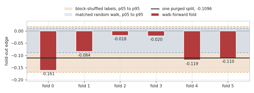
Fig. 6. Six folds, both nulls, and the single purged split as a horizontal line. Every fold sits inside at least one null band, and no fold is positive

The margin has its own trap, and section 6 of the scan exists to expose it. The analytic band sqrt(2/D) is the correct standard deviation for a margin between two unrelated prototypes. Once a classifier has absorbed a thousand correlated rows its prototypes are no longer unrelated to a typical input, so the measured spread is larger. Much larger, and the scan measures it on every row of the sample, most of which the model trained on, which is the friendliest case for the band:

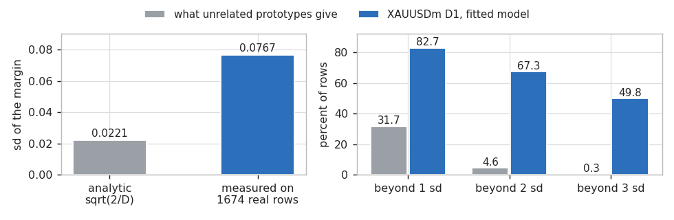
Fig. 7. On 1674 real rows the margin spreads 3.47 times wider than the closed form, and 49.8 percent of rows fall beyond three standard deviations where unrelated prototypes would give 0.3 percent

So crossing the band says the two prototypes are genuinely apart for that row. It does not say the direction is right, and any display of this number has to say so. The library still draws the band, because the scale is informative and costs nothing, but the verdict shown to a user comes from the hold-out edge instead.

The indicator

HDC_Regime.mq5 plots the margin in a subwindow with its analytic band on either side, and reports the model behind it in a panel. It is also the shortest complete example of driving the library: build the dataset, choose the training range, fit, then read the margin row by row.

   //--- the display window in CHART bar indices, and the row that opens it
   int firstDisplayBar = rates_total - InpHistoryBars;
   if(firstDisplayBar < 0)
      firstDisplayBar = 0;

   //--- copied bar i is chart bar rates_total - got + i, and a label reads
   //    horizon ahead, so the split's own purge keeps it out of the window
   int offset  = rates_total - got;
   int purge   = InpNgram + InpHorizon;
   int trainTo = -1;
   for(int r = 0; r < rows; r++)
     {
      if(offset + g_data.BarOf(r) + purge < firstDisplayBar)
         trainTo = r;
      else
         break;
     }
   if(trainTo < 200)
     {
      PrintFormat(TAG + "only %d training rows before the display window", trainTo + 1);
      return(false);
     }

   if(!g_hdc.FitRange(g_data, 0, trainTo, InpValPct, InpPasses))
     {
      PrintFormat(TAG + "fit: %s", g_hdc.Fit().note);
      return(false);
     }
   g_fit = g_hdc.Fit();
   g_haveModel = true;

Four calls, and the interesting part is the loop between them. CHDCData::Build pulls the bars and labels them, CHDC::FitRange does the purged split described earlier, CHDC::Fit returns the report the panel prints, and CHDC::MarginAt supplies each plotted point. The loop decides where training stops, and applies the same purge at a second boundary: a row may train only if its own forward label lands clear of the display window. Otherwise the newest training rows would be reading the very bars the line claims to be out of sample on. That costs eight rows.

On XAUUSDm D1 with 200 plotted bars and 1200 training bars, one recompute encodes the whole 802 to 860 row dataset and measured between 206 and 675 milliseconds across six loads, so the history depth can be generous. Between refits the line is not recomputed at all: a new bar repeats the held reading, which makes the plot a staircase rather than a curve.

The panel is where the honesty lives. It puts the hold-out accuracy next to the majority baseline it has to beat, and its verdict line states outright when it does not.

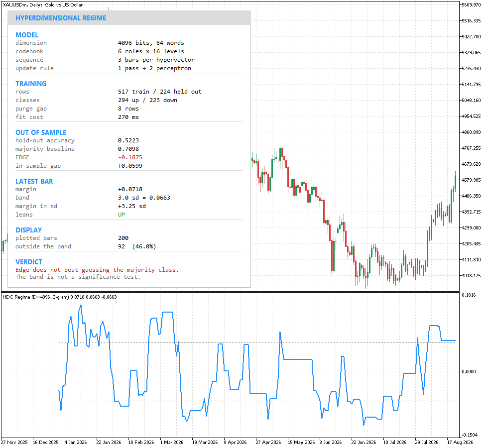
Fig. 8. HDC_Regime on XAUUSDm D1. The subwindow carries the margin between its two band lines, and the panel reports the fit behind it: a hold-out accuracy of 0.5223 against a baseline of 0.7098, and a verdict that says so

Three details in that panel are worth pointing at. The margin reads +0.0718, which is 3.25 standard deviations of the analytic band, and 92 of the 200 plotted bars are outside that band, so crossing it is a common state rather than an event and the newest bar being outside it means nothing on its own. The edge is -0.1875 while the in-sample gap is +0.0599, which is the overfit stated as a number. And the purge gap is 8 rows, separating the 224 held-out rows from the 517 the model trained on.

Cost

Every figure below came from GetMicrosecondCount taken as the minimum of several repetitions, and every range spans runs of identical code on a busier and on a quieter terminal. Reporting the spread rather than one sample is the honest form, because a stopwatch inside a running terminal is also measuring the charts, and the two ends differ by up to a factor of four for that reason alone.

Operation	Measured
One bind, D = 2048	0.055 to 0.148 us
One distance, D = 2048	0.057 to 0.229 us
One margin against both prototypes, D = 4096	0.74 to 0.76 us
Encode one record, D = 4096	70.5 to 78.0 us
One online update, D = 4096	337 to 434 us
One full fit over 1674 rows, D = 4096	425 to 555 ms

The shape of that table is the point. A record is a bundle over D bit positions of six bound levels, so encoding dominates everything else by two orders of magnitude, and the parameters that move the cost are InpNgram and InpLevels rather than anything in the classifier. A full fit is 254 to 332 microseconds per row, essentially all of it encoding. An online update encodes one row and no more, and that is what it saves: not the cost of encoding, but the cost of encoding the history again.

Conclusion

The library is complete and every level of it has been run against the sources attached here. What you can do with it now:

• Build a codebook at any dimension that is a multiple of 64, with graded level ladders whose distances match a closed form to 0 bits.
• Encode a window of bars into one hypervector through bind, bundle and permute, with quantizer ranges taken from training rows only.
• Fit a two-class model with one integer pass plus perceptron corrections, and validate it on a purged, ordered hold-out whose rows never reach the quantizer.
• Fold a new labeled bar into that model for a few hundred microseconds, and know from the test suite that, with the perceptron corrections off, the accumulator it leaves behind is bit identical to a full refit over the same rows.
• Read a decision variable against a band that is a closed-form expression rather than a permutation run, and read a panel that says when the band is not a significance test.
• Reproduce the model in Python from an exported dataset, bit for bit, and refute it with two nulls that run through the same feature path as the real data.

The finding on price data is that this model has no predictive edge on the one symbol and timeframe it was scanned over, XAUUSDm D1, at the one parameter set listed earlier; that the sign holds across six overlapping walk-forward folds there; and that it is inside both nulls. Nothing is claimed for any other market, timeframe or setting: one symbol is a hypothesis, and the scan is written so that another can be pointed at it in a single input.

Nor does the scan separate the causes. A negative edge here is consistent with the market carrying nothing this model could use, and equally consistent with the wrong six features, a label that thresholds away the moves worth predicting, a purge that leaves the trailing windows correlated, or a classifier whose capacity sits in the wrong place. What the tests establish is that the implementation is the one specified and that this configuration found no edge. Which of those is the interesting sentence the scan cannot decide, and saying so is the honest end of it. The controls bought the ability to say it at all, and only because they were built at the same time as the method.

#	Filename	Type	Description
1	HDC.mqh	Include	The facade: codebook, encoder and classifier in one object, with the purged split and the online update
2	HDCVector.mqh	Include	Packed hypervectors: bind, bundle, permute, population count and the integer distance
3	HDCRandom.mqh	Include	splitmix64 into xorshift64*, matched word for word to the Python reference
4	HDCMemory.mqh	Include	Item memory: random vectors for names, graded ladders for quantities
5	HDCEncoder.mqh	Include	Bars to records and records to sequence hypervectors, with training-only quantizer ranges
6	HDCClassifier.mqh	Include	Integer accumulators, one pass plus perceptron passes, and the margin
7	HDCStats.mqh	Include	The closed forms: noise floor, margin band, bundle capacity and the level cuts
8	HDCData.mqh	Include	Bars to six causal scale-free features, and the thresholded forward label
9	HDCPanel.mqh	Include	Panel geometry and glyph advance, so a width and the check on it are one formula
10	HDC_Test_Vector.mq5	Script	Generator conformance, the three operations, and the distance distribution
11	HDC_Test_Memory.mq5	Script	Ladder exactness, codebook independence and capacity against theory
12	HDC_Test_Classifier.mq5	Script	The online update, the noise band, the encoder, learning and a random-label control
13	HDC_Export_ForCrosscheck.mq5	Script	Dumps the whole pipeline at full precision for the Python reference to rebuild
14	HDC_Scan_Market.mq5	Script	Real bars against two nulls, walk forward, the margin band, online against batch, and cost
15	HDC_Regime.mq5	Indicator	The margin and its analytic band in a subwindow, with a panel reporting the fit behind it
16	hdc_prototype.py	Python	The blueprint the MQL5 library mirrors, with its own self-test
17	hdc_crosscheck.py	Python	Rebuilds the exported model in Python and demands bit equality
18	MQL5.zip	Archive	Archive with all project files in their subfolders; unpack it into the terminal data directory and every file lands in its required location