Diebold-Mariano Testing in MQL5: Validating Predictive Edge Across Instruments and Models

Introduction

Sooner or later you end up with two forecasters, and the question that follows is rarely asked with enough rigor: is the new one actually better, or does it just look better on the chart you happened to be staring at? Equity curves answer this poorly - two curves can cross a dozen times and still leave you guessing whether the separation is real skill or favorable noise. What's needed is a formal test on the two series of forecast errors that accounts for serial correlation and small-sample behavior before calling a difference significant.

That test exists. Diebold and Mariano built it in 1995 for comparing macroeconomic forecasters, and it travels well to trading: given two loss-differential series, it returns a statistic and a p-value saying whether the difference in accuracy is distinguishable from zero. This article implements it natively in MQL5, with Newey-West HAC variance correction and the Harvey-Leybourne-Newbold small-sample adjustment - the latter starts to matter once you're down to a few hundred bars. An EA and a subwindow indicator both run it live and show a rolling verdict.

Scope note: this article builds a comparison engine first and a trading layer second. The EA runs two forecasters side by side, computes a live rolling DM statistic, renders a color-coded verdict dashboard, and only then trades the currently-favored model's direction so the verdict carries a real trade count - the dashboard's answer is what's worth trusting; the trading logic exists to make that answer measurable, not to be a finished strategy.

Why equity curves lie to you

One terminology note: everywhere this article says "return," it means the raw bar-to-bar price change (close[t] - close[t-1]), not a percentage or log return - the DM math doesn't care which convention you use, as long as both sides of the comparison use the same one.

Comparing cumulative loss levels directly is weak: forecast errors in financial time series are heteroskedastic and autocorrelated - easy, low-volatility bars push both models' errors down together, a volatility spike does the opposite - so a naive t-test assuming independent observations will happily report significance on what's really just shared exposure to the same volatility regime. The DM test survives this by working with the loss differential series instead of loss levels, estimating its long-run variance with a heteroskedasticity-and-autocorrelation-consistent (HAC) estimator rather than the naive sample variance - the part most from-scratch implementations skip, and the part that actually makes the test trustworthy on financial data. Section 3 covers how that estimator behaves at this article's default one-step horizon.

The math: loss differentials, HAC variance, and the HLN correction

Let e1_t and e2_t be the forecast errors of Model A and Model B at bar t - realized price change minus predicted price change. Choose a loss function L(.), typically squared error for continuous forecasts, and build the loss differential d_t = L(e1_t) - L(e2_t) for every bar; a negative d_t means Model A had the lower loss. Everything downstream operates on this single series, packed into one small struct:

ENUM_DM_LOSS and DMResult

//--- Loss function types
enum ENUM_DM_LOSS
  {
   DM_LOSS_SQUARED = 0,   // (e)^2
   DM_LOSS_ABSOLUTE = 1   // |e|
  };

//--- Result container for a single DM test
struct DMResult
  {
   double            mean_diff;      // d-bar
   double            hac_variance;  // long-run variance estimate
   double            dm_stat;       // raw DM statistic
   double            hln_stat;      // Harvey-Leybourne-Newbold corrected statistic
   double            pvalue;        // two-tailed p-value (Student-t)
   int               n;                // sample size used
   int               horizon;       // forecast horizon h
   string         verdict;       // see the verdict strings table below
  };

Five verdict strings can come back; the first two are outcomes, the rest are reasons the test refused to answer at all:

Verdict string	Meaning
A_BETTER / B_BETTER	The test ran and found a statistically significant loss difference at the configured alpha
NO_SIGNIFICANT_DIFF	The test ran; the p-value cleared alpha, or the two forecasters' errors were numerically indistinguishable
INSUFFICIENT_SAMPLE	Fewer bars than the manifest's min_sample_size were available - no test was attempted
INVALID_HORIZON	horizon was zero or negative, or (less obviously) large enough relative to n that the HLN correction term itself goes negative under the radical - both are rejected explicitly rather than letting MathSqrt() return NaN
INVALID_VARIANCE	The HAC variance estimate came back negative - a numerically invalid result, not a "no difference" one

The loss differential is computed bar by bar as d_t = L(e1_t) - L(e2_t), using whichever loss function was chosen:

DM_LossDifferential

//+------------------------------------------------------------------+
//| Compute per-bar loss differential d_t = L(e1_t) - L(e2_t)        |
//+------------------------------------------------------------------+
void DM_LossDifferential(const double &errA[], const double &errB[], const ENUM_DM_LOSS loss_type,
                         double &d_out[])
  {
   int n = MathMin(ArraySize(errA), ArraySize(errB));
   ArrayResize(d_out, n);
   for(int i = 0; i < n; i++)
     {
       double la, lb;
       if(loss_type == DM_LOSS_SQUARED)
         {
           la = errA[i] * errA[i];
           lb = errB[i] * errB[i];
         }
       else
         {
           la = MathAbs(errA[i]);
           lb = MathAbs(errB[i]);
         }
       d_out[i] = la - lb;
     }
  }

The test statistic is built from the sample mean of d_t divided by an estimate of its standard error: DM = d_bar / sqrt(V_hat / T), where V_hat is the long-run variance of d_bar. Rather than the naive sample variance of d_t, the HAC estimator sums the autocovariances at every lag up to h-1 (h being the forecast horizon), weighted down with a Bartlett kernel so distant lags contribute less. The autocovariance at a given lag is a small helper function on its own:

DM_Autocovariance

//+------------------------------------------------------------------+
//| Sample autocovariance at lag k for a zero-lag-demeaned series    |
//+------------------------------------------------------------------+
double DM_Autocovariance(const double &d[], const double mean, const int k)
  {
   int n = ArraySize(d);
   if(k >= n)
       return(0.0);
   double sum = 0.0;
   for(int t = k; t < n; t++)
       sum += (d[t] - mean) * (d[t - k] - mean);
   return(sum / n);
  }

DM_HACVariance

//+------------------------------------------------------------------+
//| Bartlett-kernel HAC (Newey-West) long-run variance of d-bar      |
//| lag_max = h - 1, per Diebold & Mariano (1995)                    |
//+------------------------------------------------------------------+
double DM_HACVariance(const double &d[], const int horizon)
  {
   int n = ArraySize(d);
   if(n <= 1)
       return(0.0);

   double mean = 0.0;
   for(int i = 0; i < n; i++)
       mean += d[i];
   mean /= n;

   int lag_max = MathMax(0, horizon - 1);
   //--- guard: lag window cannot exceed available sample
   lag_max = MathMin(lag_max, n - 1);

   double gamma0 = DM_Autocovariance(d, mean, 0);
   double var_sum = gamma0;

   //--- h == 1 collapses to plain sample variance, no Bartlett terms needed
   for(int k = 1; k <= lag_max; k++)
     {
       double w = 1.0 - (double)k / (double)horizon;   // Bartlett kernel weight
       double gamma_k = DM_Autocovariance(d, mean, k);
       var_sum += 2.0 * w * gamma_k;
     }
   return(var_sum);
  }

The p-value and critical-value bands need a Student-t distribution, but not every MetaTrader install ships the Standard Library's Math\Stat\Student.mqh, so the library carries its own CDF and quantile instead, through the standard regularized incomplete beta route:

DM_StudentCDF / DM_StudentQuantile (with their incomplete-beta helpers)

double DM_LogGamma(const double x)
  {
   double cof[6] =
     {
       76.18009172947146, -86.50532032941677, 24.01409824083091,
       -1.231739572450155, 0.1208650973866179e-2, -0.5395239384953e-5
     };
   double y = x;
   double tmp = x + 5.5;
   tmp -= (x + 0.5) * MathLog(tmp);
   double ser = 1.000000000190015;
   for(int j = 0; j < 6; j++)
     {
       y += 1.0;
       ser += cof[j] / y;
     }
   return(-tmp + MathLog(2.5066282746310005 * ser / x));
  }

double DM_BetaCF(const double x, const double a, const double b)
  {
   const int max_iter = 200;
   const double eps     = 3.0e-12;
   const double fpmin   = 1.0e-300;

   double qab = a + b;
   double qap = a + 1.0;
   double qam = a - 1.0;
   double c = 1.0;
   double d = 1.0 - qab * x / qap;
   if(MathAbs(d) < fpmin) d = fpmin;
   d = 1.0 / d;
   double h = d;

   for(int m = 1; m <= max_iter; m++)
     {
       double m2 = 2.0 * m;
       double aa = m * (b - m) * x / ((qam + m2) * (a + m2));
       d = 1.0 + aa * d;   if(MathAbs(d) < fpmin) d = fpmin;
       c = 1.0 + aa / c;   if(MathAbs(c) < fpmin) c = fpmin;
       d = 1.0 / d;
       h *= d * c;

       aa = -(a + m) * (qab + m) * x / ((a + m2) * (qap + m2));
       d = 1.0 + aa * d;   if(MathAbs(d) < fpmin) d = fpmin;
       c = 1.0 + aa / c;   if(MathAbs(c) < fpmin) c = fpmin;
       d = 1.0 / d;
       double del = d * c;
       h *= del;

       if(MathAbs(del - 1.0) < eps)
         break;
     }
   return(h);
  }

double DM_IncompleteBeta(const double x, const double a, const double b)
  {
   if(x <= 0.0) return(0.0);
   if(x >= 1.0) return(1.0);

   double bt = MathExp(DM_LogGamma(a + b) - DM_LogGamma(a) - DM_LogGamma(b) +
               a * MathLog(x) + b * MathLog(1.0 - x));

   if(x < (a + 1.0) / (a + b + 2.0))
       return(bt * DM_BetaCF(x, a, b) / a);
   else
       return(1.0 - bt * DM_BetaCF(1.0 - x, b, a) / b);
  }

//+------------------------------------------------------------------+
//| P(T <= t) for a Student-t distribution with the given df         |
//+------------------------------------------------------------------+
double DM_StudentCDF(const double t, const double df)
  {
   double x   = df / (df + t * t);
   double ib = DM_IncompleteBeta(x, df / 2.0, 0.5);
   return(t > 0.0 ? 1.0 - 0.5 * ib : 0.5 * ib);
  }

//+------------------------------------------------------------------+
//| Inverse CDF via bisection - monotone in t, robust for any df      |
//+------------------------------------------------------------------+
double DM_StudentQuantile(const double p, const double df)
  {
   double lo = -100.0, hi = 100.0;
   for(int i = 0; i < 200; i++)
     {
       double mid = 0.5 * (lo + hi);
       if(DM_StudentCDF(mid, df) < p)
         lo = mid;
       else
         hi = mid;
     }
   return(0.5 * (lo + hi));
  }

The CDF comes from the regularized incomplete beta function, and the quantile from bisection on it, which was spot-checked against scipy.stats.t on a handful of df/p combinations during development and tracked closely. Fig. 2 shows how the Bartlett weights decay for different horizons. At h = 1 the sum collapses entirely - no lag terms survive, and the estimator reduces to plain sample variance. That's a deliberate edge case, not an oversight: one-step-ahead forecasts (the default in this article) don't have the overlapping-forecast autocorrelation that longer horizons introduce. What that protects against, at any horizon, is specifically the serial dependence overlapping multi-step forecasts induce - it isn't a general fix for every source of autocorrelation a loss differential could have, so volatility-clustering-driven dependence unrelated to forecast overlap can still sit uncorrected at h=1.

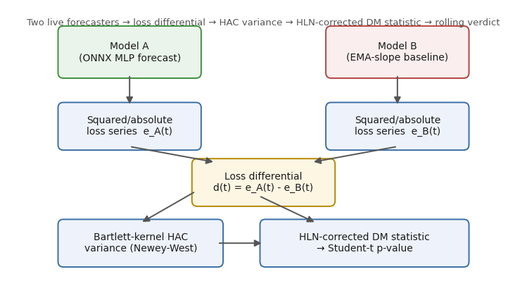
Fig. 1. Data flow from two live forecasters through the loss differential, HAC variance, and HLN-corrected DM statistic, into the rolling verdict dashboard.

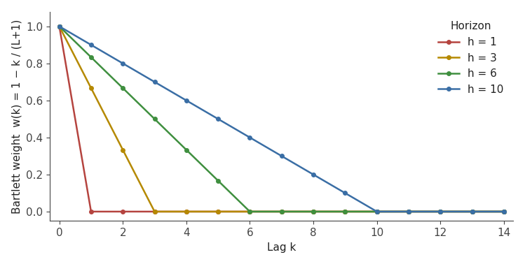
Fig. 2. Bartlett kernel weights across lags for several forecast horizons h. At h=1 the sum has no lag terms; longer horizons let more distant autocovariances contribute, tapering linearly to zero.

The raw DM statistic, tested against a standard normal distribution, is only valid asymptotically, with hundreds or thousands of independent observations - a luxury MetaTrader backtests rarely give cleanly. Harvey, Leybourne, and Newbold's 1997 correction fixes this by rescaling the statistic and testing it against a Student-t distribution with n-1 degrees of freedom instead. Its practical effect scales with the horizon: at h=1 the h(h-1) term vanishes and the rescaling factor is close to 1 (roughly 0.998 at n=250), growing more consequential as h increases. Everything above comes together in one function that's the actual entry point the EA and the indicator both call:

DM_RunTest

//+------------------------------------------------------------------+
//| Full Diebold-Mariano test with HLN small-sample correction       |
//+------------------------------------------------------------------+
bool DM_RunTest(const double &errA[], const double &errB[], const int horizon,
          const ENUM_DM_LOSS loss_type, DMResult &result,
          const int min_sample_size = 30, const double significance_alpha = 0.10)
  {
   result.horizon = horizon;

   //--- a horizon of zero or less breaks both the truncation lag (h-1) and
   //--- the HLN correction below, so it's rejected before touching the data
   if(horizon <= 0)
     {
       result.n = 0;
       result.verdict = "INVALID_HORIZON";
       result.mean_diff = 0.0;
       result.hac_variance = 0.0;
       result.dm_stat = 0.0;
       result.hln_stat = 0.0;
       result.pvalue = 1.0;
       return(false);
     }

   double d[];
   DM_LossDifferential(errA, errB, loss_type, d);
   int n = ArraySize(d);
   result.n = n;

   //--- insufficient sample size for asymptotic validity, driven by the
   //--- manifest's min_sample_size rather than a hardcoded literal
   if(n < min_sample_size)
     {
       result.verdict = "INSUFFICIENT_SAMPLE";
       result.mean_diff = 0.0;
       result.hac_variance = 0.0;
       result.dm_stat = 0.0;
       result.hln_stat = 0.0;
       result.pvalue = 1.0;
       return(false);
     }

   double mean = 0.0;
   for(int i = 0; i < n; i++)
       mean += d[i];
   mean /= n;

   double long_run_var = DM_HACVariance(d, horizon);
   result.mean_diff     = mean;
   result.hac_variance = long_run_var;

   //--- a negative long-run variance is a numerically invalid HAC estimate -
   //--- the Bartlett-kernel sum isn't guaranteed positive semi-definite in
   //--- finite samples - and must not be folded into "no difference" below
   if(long_run_var < 0.0)
     {
       result.dm_stat  = 0.0;
       result.hln_stat = 0.0;
       result.pvalue   = 1.0;
       result.verdict  = "INVALID_VARIANCE";
       return(false);
     }

   //--- guard against near-zero denominator (degenerate/identical forecasters);
   //--- this is a legitimate case, unlike the negative-variance one above
   double denom = long_run_var / (double)n;
   if(denom < 1e-12)
     {
       result.dm_stat  = 0.0;
       result.hln_stat = 0.0;
       result.pvalue   = 1.0;
       result.verdict  = "NO_SIGNIFICANT_DIFF";
       return(true);
     }

   double dm_raw = mean / MathSqrt(denom);

   //--- Harvey, Leybourne & Newbold (1997): S* = S * sqrt[(n+1-2h+h(h-1)/n)/n] -
   //--- the h(h-1) term is divided by n BEFORE being summed with (n+1-2h)
   double correction_numerator = (double)(n + 1 - 2 * horizon) +
                                     (double)(horizon * (horizon - 1)) / (double)n;

   //--- for a horizon large relative to n, correction_numerator can go negative -
   //--- that would hand MathSqrt() a negative argument and silently return NaN
   //--- straight into dm_hln, pvalue and verdict, so it must fail explicitly
   if(correction_numerator <= 0.0)
     {
       result.dm_stat  = dm_raw;
       result.hln_stat = 0.0;
       result.pvalue   = 1.0;
       result.verdict  = "INVALID_HORIZON";
       return(false);
     }

   double hln_factor = MathSqrt(correction_numerator / (double)n);
   double dm_hln = dm_raw * hln_factor;

   result.dm_stat  = dm_raw;
   result.hln_stat = dm_hln;

   //--- two-tailed p-value against Student-t(n-1), self-contained CDF above
   double cdf = DM_StudentCDF(MathAbs(dm_hln), (double)(n - 1));
   result.pvalue = 2.0 * (1.0 - cdf);

   if(result.pvalue > significance_alpha)
       result.verdict = "NO_SIGNIFICANT_DIFF";
   else
       result.verdict = (mean < 0.0) ? "A_BETTER" : "B_BETTER";   // d = L(A) - L(B); negative mean => A has lower loss

   return(true);
  }

Three things worth calling out in that signature. The h(h-1) term inside the square root must be divided by n before being added to (n+1-2h) - get the order wrong and the bug is invisible at h=1 (where h(h-1)=0) but drifts from the real correction at longer horizons. correction_numerator isn't guaranteed positive: for a horizon large relative to n it can go negative, which would hand MathSqrt() a negative argument and silently return NaN into hln_stat, pvalue, and verdict - the explicit check above catches that and returns INVALID_HORIZON instead. And min_sample_size / significance_alpha are manifest-driven parameters, not hardcoded literals, which matters at the sample sizes a few months of M5 data with a short rolling window actually gives you: without the HLN correction you'll over-reject the null and convince yourself of edges that aren't there.

Choosing a loss function: squared vs absolute error

The DM test doesn't care which loss function you pick, as long as both sides use the same one - the math works identically for squared or absolute error, since the test only ever looks at the differential d_t (that's the branch inside DM_LossDifferential() above). The choice still matters practically: squared error punishes large misses disproportionately, which usually suits a position-sizing layer since an occasional wildly wrong prediction is more dangerous than a slightly higher average miss; absolute error treats every unit of error the same, which suits logic that only cares about directional correctness and shouldn't let a handful of volatility-spike bars dominate.

The manifest exposes this as a single loss_type field rather than a recompile-required constant, so you can rerun the same error logs through both and see if your conclusion survives the choice. If Model A wins under squared error but loses under absolute error, that's not a contradiction - it wins on average but loses on typical-case accuracy, usually by flagging rare large moves better and routine ones worse.

Two concrete forecasters

To make the test tangible rather than abstract, the EA runs two forecasters against each other continuously:

Model A - ONNX regression forecaster. An 8-feature model predicting next-bar price change, exported through a standard sklearn-to-ONNX pipeline: three ATR-normalized lagged price changes, ATR-to-price ratio, scaled RSI, ATR-normalized MACD histogram, EMA slope, and log-scaled real volume.

Model B - EMA-slope baseline. The slope of a 20-period EMA, used directly as the next-bar price-change prediction - no ML, the benchmark a more complex model has to actually beat.

Both models predict at bar close t the price change realized at t+1. The EA waits one bar, computes both realized errors, and appends them to two growing history arrays that the static and rolling DM tests both operate on. The EA and the indicator in Section 8 call the exact same two functions below rather than each keeping its own copy:

DM_BuildFeatureVector

//+------------------------------------------------------------------+
//| Shared 8-feature builder for the ONNX forecaster (Model A)       |
//| Used identically by the EA and the indicator so both ever run    |
//| the same model on the same feature contract - no separate,       |
//| drifting copy of this logic in each file.                        |
//+------------------------------------------------------------------+
bool DM_BuildFeatureVector(const string symbol, const int h_ema, const int h_atr,
                         const int h_rsi, const int h_macd, const int shift,
                         float &features[])
  {
   double close_arr[], atr_arr[], rsi_arr[], macd_main[], macd_signal[], ema_arr[];

   if(CopyClose(symbol, PERIOD_CURRENT, shift, 5, close_arr) < 5)
       return(false);
   if(CopyBuffer(h_atr, 0, shift, 2, atr_arr) < 2)
       return(false);
   if(CopyBuffer(h_rsi, 0, shift, 2, rsi_arr) < 2)
       return(false);
   if(CopyBuffer(h_macd, 0, shift, 2, macd_main) < 2)
       return(false);
   if(CopyBuffer(h_macd, 1, shift, 2, macd_signal) < 2)
       return(false);
   if(CopyBuffer(h_ema, 0, shift, 3, ema_arr) < 3)
       return(false);

   //--- volume_real, not tick_volume: falls back to tick volume only when
   //--- the broker feed genuinely has no real-volume data for this bar
   MqlRates rates[];
   if(CopyRates(symbol, PERIOD_CURRENT, shift, 2, rates) < 2)
       return(false);
   double vol_real = (rates[0].tick_volume > 0) ? (double)rates[0].tick_volume : 1.0;
   if(rates[0].real_volume > 0)
       vol_real = (double)rates[0].real_volume;

   double atr_now = MathMax(atr_arr[1], 1e-8);   // divide-by-zero guard

   ArrayResize(features, NUM_FEATURES);
   features[0] = (float)((close_arr[4] - close_arr[3]) / atr_now);   // return lag1, ATR-normalized
   features[1] = (float)((close_arr[3] - close_arr[2]) / atr_now);   // return lag2
   features[2] = (float)((close_arr[2] - close_arr[1]) / atr_now);   // return lag3
   features[3] = (float)(atr_now / close_arr[4]);            // ATR normalized by price
   features[4] = (float)(rsi_arr[1] / 100.0);             // RSI scaled 0-1
   features[5] = (float)((macd_main[1] - macd_signal[1]) / atr_now); // MACD histogram, ATR-normalized
   features[6] = (float)((ema_arr[2] - ema_arr[0]) / (2.0 * atr_now)); // EMA slope, ATR-normalized
   features[7] = (float)MathLog(1.0 + vol_real / 1000.0);       // log-scaled real volume

   //--- reject a feature vector carrying NaN/Inf before it ever reaches the
   //--- ONNX model - a bad upstream indicator tick is more useful as a
   //--- skipped bar than as silently-propagated garbage in the error history
   for(int i = 0; i < NUM_FEATURES; i++)
       if(!MathIsValidNumber(features[i]))
           return(false);

   return(true);
  }

Every feature is checked with MathIsValidNumber() before the vector is returned, so a NaN/Inf feature from a bad tick, division edge case, or ONNX warm-up gap becomes a skipped bar instead of silently corrupting the error history - the same check applies to ONNX's own output in ForecastModelA().

DM_ForecastModelB

//+------------------------------------------------------------------+
//| Shared Model B forecast: raw EMA slope, used directly as the     |
//| next-bar return prediction (no ML, no rescaling) - this is the   |
//| deliberately simple momentum-continuation baseline               |
//+------------------------------------------------------------------+
double DM_ForecastModelB(const int h_ema, const int shift)
  {
   double ema_arr[];
   if(CopyBuffer(h_ema, 0, shift, 3, ema_arr) < 3)
       return(0.0);
   return((ema_arr[2] - ema_arr[0]) / 2.0);
  }

Model B stays the raw EMA slope with no rescaling - an ATR-normalize-then-multiply-back step would be algebraically a no-op, just dressing the same number up with a misleading comment.

Feature-contract self-testing and ONNX wiring

Any ONNX-driven EA needs the same discipline: the feature count is a compile-time constant (NUM_FEATURES, defined once in DMTest.mqh and shared by the EA and indicator), and at OnInit() the EA builds one live feature vector and checks its width against it, so a future edit that silently drops or adds a feature fails loudly at startup instead of feeding a misaligned vector for weeks.

The EA's feature builder and ONNX forecast call are thin wrappers around the shared functions above:

BuildFeatureVector / ForecastModelA (DM_Test_EA.mq5)

//+------------------------------------------------------------------+
//| Build the 8-feature vector for the ONNX forecaster                |
//| Thin wrapper: the actual feature math lives in DM_BuildFeature-   |
//| Vector() in DMTest.mqh so the indicator uses the exact same       |
//| contract instead of a second, hand-copied version.                |
//+------------------------------------------------------------------+
bool BuildFeatureVector(const int shift, float &features[])
  {
   return(DM_BuildFeatureVector(_Symbol, g_h_ema, g_h_atr, g_h_rsi, g_h_macd, shift, features));
  }

//+------------------------------------------------------------------+
//| Model A forecast via ONNX                                        |
//+------------------------------------------------------------------+
double ForecastModelA(const int shift)
  {
   float features[];
   if(!BuildFeatureVector(shift, features))
       return(0.0);

   float input_data[1][NUM_FEATURES];
   for(int i = 0; i < NUM_FEATURES; i++)
       input_data[0][i] = features[i];

   float output_data[1][1];
   if(!OnnxRun(g_onnx_handle, ONNX_DEFAULT, input_data, output_data))
     {
       Print("DM_Test_EA: OnnxRun failed, error ", GetLastError());
       return(0.0);
     }
   if(!MathIsValidNumber(output_data[0][0]))
     {
       Print("DM_Test_EA: ONNX returned a non-finite value, treating as no forecast.");
       return(0.0);
     }
   return((double)output_data[0][0]);
  }

The self-test that guards this contract builds one throwaway feature vector at load time and compares its width to the declared constant - if BuildFeatureVector() ever changes shape without the constant being updated too, this is what stops the EA cold instead of letting it trade on garbage:

SelfTestFeatureContract

//+------------------------------------------------------------------+
//| Feature-contract self-test: declared width vs actual output      |
//+------------------------------------------------------------------+
bool SelfTestFeatureContract()
  {
   float test_features[];
   if(!BuildFeatureVector(1, test_features))
     {
       Print("DM_Test_EA: SelfTest - could not build a sample feature vector yet (insufficient history).");
       return(true); // not fatal at chart-load, retried on first real bar
     }
   int actual_width = ArraySize(test_features);
   if(actual_width != NUM_FEATURES)
     {
       PrintFormat("DM_Test_EA: FATAL feature contract mismatch - declared NUM_FEATURES=%d, builder produced %d.",
               NUM_FEATURES, actual_width);
       return(false);
     }
   Print("DM_Test_EA: feature contract self-test passed (", NUM_FEATURES, " features).");
   return(true);
  }

The ONNX model itself is wired with fixed batch-size-1 input and output shapes set explicitly before any inference call, rather than relying on the model's declared shape metadata. That happens inside OnInit(), alongside creating the four indicator handles the feature builder needs and the self-test above:

OnInit (DM_Test_EA.mq5)

//+------------------------------------------------------------------+
//| Expert initialization                                            |
//+------------------------------------------------------------------+
int OnInit()
  {
   LoadManifest();

   g_h_ema  = iMA(_Symbol, PERIOD_CURRENT, InpEmaPeriod, 0, MODE_EMA, PRICE_CLOSE);
   g_h_atr  = iATR(_Symbol, PERIOD_CURRENT, InpAtrPeriod);
   g_h_rsi  = iRSI(_Symbol, PERIOD_CURRENT, InpRsiPeriod, PRICE_CLOSE);
   g_h_macd = iMACD(_Symbol, PERIOD_CURRENT, InpMacdFast, InpMacdSlow, InpMacdSignal, PRICE_CLOSE);

   if(g_h_ema == INVALID_HANDLE || g_h_atr == INVALID_HANDLE ||
     g_h_rsi == INVALID_HANDLE || g_h_macd == INVALID_HANDLE)
     {
       Print("DM_Test_EA: failed to create indicator handles.");
       return(INIT_FAILED);
     }

   //--- ONNX_COMMON_FOLDER: the Strategy Tester runs each EA inside its own
   //--- private per-agent MQL5\Files sandbox, not the live terminal's data
   //--- folder - loading from the shared Common\Files folder instead means
   //--- the model resolves the same whether this runs live or under a tester agent
   g_onnx_handle = OnnxCreate(InpOnnxModel, ONNX_COMMON_FOLDER);
   if(g_onnx_handle == INVALID_HANDLE)
     {
       PrintFormat("DM_Test_EA: failed to load ONNX model '%s', error %d.", InpOnnxModel, GetLastError());
       return(INIT_FAILED);
     }

   const long input_shape[]  = {1, NUM_FEATURES};
   const long output_shape[] = {1, 1};
   if(!OnnxSetInputShape(g_onnx_handle, 0, input_shape))
     {
       Print("DM_Test_EA: OnnxSetInputShape failed.");
       return(INIT_FAILED);
     }
   if(!OnnxSetOutputShape(g_onnx_handle, 0, output_shape))
     {
       Print("DM_Test_EA: OnnxSetOutputShape failed.");
       return(INIT_FAILED);
     }

   if(!SelfTestFeatureContract())
       return(INIT_FAILED);

   if(!g_canvas.CreateBitmapLabel("DM_Dashboard", 20, 20, 340, 110, COLOR_FORMAT_ARGB_NORMALIZE))
     {
       Print("DM_Test_EA: canvas creation failed.");
       return(INIT_FAILED);
     }

   ArrayResize(g_pred_a, 0);
   ArrayResize(g_pred_b, 0);
   ArrayResize(g_err_a, 0);
   ArrayResize(g_err_b, 0);
   ArrayResize(g_actual_ret, 0);

   DrawDashboard("Awaiting sample...", clrGray);
   return(INIT_SUCCEEDED);
  }

The volume feature uses volume_real rather than tick volume, falling back to tick volume only when a bar genuinely has no real-volume data.

One detail worth flagging: the EA never retrains or refits either forecaster during a run - Model A's ONNX weights are frozen at export time, Model B's EMA parameters are fixed. This is non-negotiable for the DM test to mean anything: letting one model adapt mid-test contaminates the loss differential with a structural break the HAC estimator isn't designed to absorb.

The EA's rolling test and on-chart dashboard

A single static DM test over an entire backtest tells you whether one model was better on average across the whole window, but it hides regime changes - Model A might have dominated for the first half and then degraded. On every closed bar, OnTick() appends both models' realized error to a running history and, every g_dash_refresh bars, runs both the full-sample test and a rolling-window test against just the trailing g_window bars:

OnTick (DM_Test_EA.mq5)

//+------------------------------------------------------------------+
//| Expert tick - process strictly on new bar close                  |
//+------------------------------------------------------------------+
void OnTick()
  {
   datetime cur_bar_time = iTime(_Symbol, PERIOD_CURRENT, 0);
   if(cur_bar_time == g_last_bar_time)
       return;
   g_last_bar_time = cur_bar_time;

   // shift=1 is the just-closed bar; we score its ALREADY-REALIZED outcome using
   // the forecast available for it back at shift=2 - a backward-looking pair for
   // the error history, kept separate from the live forecast used for trading below
   double predA = ForecastModelA(2);
   double predB = ForecastModelB(2);

   double close1[], close2[];
   if(CopyClose(_Symbol, PERIOD_CURRENT, 1, 1, close1) < 1) return;
   if(CopyClose(_Symbol, PERIOD_CURRENT, 2, 1, close2) < 1) return;
   double realized_ret = close1[0] - close2[0];

   double errA = realized_ret - predA;
   double errB = realized_ret - predB;

   int n = ArraySize(g_err_a);
   ArrayResize(g_pred_a, n + 1);     g_pred_a[n] = predA;
   ArrayResize(g_pred_b, n + 1);     g_pred_b[n] = predB;
   ArrayResize(g_err_a, n + 1);       g_err_a[n] = errA;
   ArrayResize(g_err_b, n + 1);       g_err_b[n] = errB;
   ArrayResize(g_actual_ret, n + 1);   g_actual_ret[n] = realized_ret;

   g_bars_since_refresh++;
   if(g_bars_since_refresh < g_dash_refresh)
       return;
   g_bars_since_refresh = 0;

   DM_RunTest(g_err_a, g_err_b, g_horizon, g_loss_type, g_static_result, g_min_sample, g_alpha);
   DM_RunRolling(g_err_a, g_err_b, g_window, g_horizon, g_loss_type, g_rolling_result, g_min_sample, g_alpha);

   string verdict_label = g_rolling_result.verdict;
   StringReplace(verdict_label, "_", " ");
   DrawDashboard(verdict_label, VerdictColor(g_rolling_result.verdict));

   // Trading uses a SEPARATE, live forecast for the bar still ahead (built from
   // shift=1, "as of the bar that just closed"), not the shift=2 forecast above -
   // that one scored a bar that already finished and is stale for a trade about
   // to be opened on the next one
   double liveA = ForecastModelA(1);
   double liveB = ForecastModelB(1);
   ManageTrading(liveA, liveB);
  }

Two forecasts are built here, not one: predA/predB at shift=2 score the bar that just closed, feeding the error history and the DM test, while liveA/liveB at shift=1 build a fresh forecast for the bar still ahead - the only pair ManageTrading() sees, since trading on the stale shift=2 pair would mean acting on an already-finished bar. ManageTrading() itself gives this a real trade count: flat-only entries in the winning model's direction, ATR-based SL/TP clamped to the broker's real stop-distance and margin limits, no reaction to a mid-trade signal flip. Full listing in DM_Test_EA.mq5.

DM_RunRolling() is a thin slicer around DM_RunTest(): it takes the tail of the history array and runs the same test on just that window, turning a single full-sample number into something that tracks a regime change:

DM_RunRolling

//+------------------------------------------------------------------+
//| Rolling-window wrapper: slices the tail of a vector-backed       |
//| history buffer and runs DM_RunTest on just that window           |
//+------------------------------------------------------------------+
bool DM_RunRolling(const double &errA_full[], const double &errB_full[], const int window,
              const int horizon, const ENUM_DM_LOSS loss_type, DMResult &result,
              const int min_sample_size = 30, const double significance_alpha = 0.10)
  {
   int total = MathMin(ArraySize(errA_full), ArraySize(errB_full));
   int start = MathMax(0, total - window);
   int len   = total - start;

   double slice_a[], slice_b[];
   ArrayResize(slice_a, len);
   ArrayResize(slice_b, len);
   for(int i = 0; i < len; i++)
     {
       slice_a[i] = errA_full[start + i];
       slice_b[i] = errB_full[start + i];
     }
   return(DM_RunTest(slice_a, slice_b, horizon, loss_type, result, min_sample_size, significance_alpha));
  }

That rolling statistic drives a small CCanvas dashboard: green when Model A is significantly better, red when Model B is, gray when indistinguishable, darker gray while the sample is still too small to say anything:

DrawDashboard / VerdictColor

//+------------------------------------------------------------------+
//| Draw the color-coded rolling verdict dashboard via CCanvas       |
//+------------------------------------------------------------------+
void DrawDashboard(const string verdict_text, const color bg_color)
  {
   g_canvas.Erase(ColorToARGB(bg_color, 220));
   g_canvas.FontSet("Consolas", -140, FW_BOLD);
   g_canvas.TextOut(10, 8, "DM Monitor: A (ONNX) vs B (EMA-slope)", ColorToARGB(clrWhite, 255));
   g_canvas.FontSet("Consolas", -120, FW_NORMAL);
   g_canvas.TextOut(10, 32, StringFormat("Static  DM=%.3f  HLN=%.3f  p=%.4f",
               g_static_result.dm_stat, g_static_result.hln_stat, g_static_result.pvalue),
               ColorToARGB(clrWhite, 255));
   g_canvas.TextOut(10, 52, StringFormat("Rolling DM=%.3f  HLN=%.3f  p=%.4f  n=%d",
               g_rolling_result.dm_stat, g_rolling_result.hln_stat, g_rolling_result.pvalue, g_rolling_result.n),
               ColorToARGB(clrWhite, 255));
   g_canvas.FontSet("Consolas", -150, FW_BOLD);
   g_canvas.TextOut(10, 80, "Verdict: " + verdict_text, ColorToARGB(clrWhite, 255));
   g_canvas.Update();
  }

color VerdictColor(const string verdict)
  {
   if(verdict == "A_BETTER")
       return(clrForestGreen);
   if(verdict == "B_BETTER")
       return(clrFireBrick);
   if(verdict == "INSUFFICIENT_SAMPLE")
       return(clrDarkSlateGray);
   return(clrSlateGray); // NO_SIGNIFICANT_DIFF
  }

The parameters that drive all this - horizon, rolling window, loss function, significance alpha, and dashboard refresh cadence - are read from dm_manifest.json at OnInit() through a plain key:value scan, no external DLL or JSON library needed, so the same compiled binary retunes without a recompile:

LoadManifest / LoadManifestValue

//+------------------------------------------------------------------+
//| Manifest loader - simple key:value JSON scan, no external DLL    |
//+------------------------------------------------------------------+
bool LoadManifestValue(const string &raw, const string key, string &value_out)
  {
   int pos = StringFind(raw, "\"" + key + "\"");
   if(pos < 0)
       return(false);
   int colon = StringFind(raw, ":", pos);
   int comma = StringFind(raw, ",", colon);
   int brace = StringFind(raw, "}", colon);
   int end = (comma >= 0 && (comma < brace || brace < 0)) ? comma : brace;
   if(colon < 0 || end < 0)
       return(false);
   string v = StringSubstr(raw, colon + 1, end - colon - 1);
   StringReplace(v, "\"", "");
   StringReplace(v, " ", "");
   StringReplace(v, "\n", "");
   StringReplace(v, "\r", "");
   value_out = v;
   return(true);
  }

void LoadManifest()
  {
   g_horizon       = InpHorizon;
   g_window        = InpRollingWindow;
   g_min_sample   = InpMinSample;
   g_alpha         = InpSignificanceAlpha;
   g_loss_type    = InpLossType;
   g_dash_refresh = InpDashboardRefresh;

   int fh = FileOpen(InpManifestFile, FILE_READ | FILE_TXT | FILE_ANSI | FILE_COMMON);
   if(fh == INVALID_HANDLE)
       fh = FileOpen(InpManifestFile, FILE_READ | FILE_TXT | FILE_ANSI);
   if(fh == INVALID_HANDLE)
     {
       PrintFormat("DM_Test_EA: manifest not found (%s), using input defaults.", InpManifestFile);
       return;
     }

   string raw = "";
   while(!FileIsEnding(fh))
       raw += FileReadString(fh) + "\n";
   FileClose(fh);

   string v;
   if(LoadManifestValue(raw, "forecast_horizon_h", v))    g_horizon       = (int)StringToInteger(v);
   if(LoadManifestValue(raw, "rolling_window_bars", v))   g_window        = (int)StringToInteger(v);
   if(LoadManifestValue(raw, "min_sample_size", v))      g_min_sample   = (int)StringToInteger(v);
   if(LoadManifestValue(raw, "significance_alpha", v))   g_alpha        = StringToDouble(v);
   if(LoadManifestValue(raw, "dashboard_refresh_bars", v)) g_dash_refresh = (int)StringToInteger(v);
   if(LoadManifestValue(raw, "loss_type", v))
       g_loss_type = (v == "ABSOLUTE") ? DM_LOSS_ABSOLUTE : DM_LOSS_SQUARED;

   PrintFormat("DM_Test_EA: manifest loaded - h=%d window=%d min_n=%d loss=%s",
             g_horizon, g_window, g_min_sample, (g_loss_type == DM_LOSS_SQUARED ? "SQUARED" : "ABSOLUTE"));
  }

Fields read are forecast_horizon_h, rolling_window_bars, min_sample_size, significance_alpha, loss_type (SQUARED or ABSOLUTE), and (EA only) dashboard_refresh_bars; the manifest also documents the period settings the model was built against, but those are documentation-only - the loader never reads them back into the running periods. Any missing or unrecognized field falls back silently to the EA's own input defaults with no per-field warning, so a config typo never crashes the EA but can leave it quietly running on defaults instead of what you meant to change.

The subwindow indicator: a genuinely rolling recalculation

DM_RollingMonitor.mq5 plots the rolling HLN-corrected DM statistic as a line in its own subwindow against two-tailed critical-value bands, so you see the whole comparison history at a glance instead of one live number off the dashboard. As a separate process it can't read the EA's in-memory error arrays, so it reconstructs both forecasters' error history itself, using its own ONNX and indicator handles built with the same periods - and the same dm_manifest.json - as the EA:

OnInit (DM_RollingMonitor.mq5)

int OnInit()
  {
   LoadManifest();

   SetIndexBuffer(0, BufDM, INDICATOR_DATA);
   SetIndexBuffer(1, BufUpperCrit, INDICATOR_DATA);
   SetIndexBuffer(2, BufLowerCrit, INDICATOR_DATA);
   //--- deliberately not series: OnCalculate() below walks forward,
   //--- index-aligned with the non-series time[]/close[] arrays

   g_h_ema  = iMA(_Symbol, PERIOD_CURRENT, InpEmaPeriod, 0, MODE_EMA, PRICE_CLOSE);
   g_h_atr  = iATR(_Symbol, PERIOD_CURRENT, InpAtrPeriod);
   g_h_rsi  = iRSI(_Symbol, PERIOD_CURRENT, InpRsiPeriod, PRICE_CLOSE);
   g_h_macd = iMACD(_Symbol, PERIOD_CURRENT, InpMacdFast, InpMacdSlow, InpMacdSignal, PRICE_CLOSE);

   if(g_h_ema == INVALID_HANDLE || g_h_atr == INVALID_HANDLE ||
     g_h_rsi == INVALID_HANDLE || g_h_macd == INVALID_HANDLE)
     {
       Print("DM_RollingMonitor: failed to create indicator handles.");
       return(INIT_FAILED);
     }

   //--- ONNX_COMMON_FOLDER: same reasoning as DM_Test_EA.mq5 - this indicator
   //--- also runs inside a tester-agent sandbox with its own private
   //--- MQL5\Files, so the model has to come from the shared Common folder
   g_onnx_handle = OnnxCreate(InpOnnxModel, ONNX_COMMON_FOLDER);
   if(g_onnx_handle == INVALID_HANDLE)
     {
       PrintFormat("DM_RollingMonitor: ONNX model load failed, error %d.", GetLastError());
       return(INIT_FAILED);
     }

   const long input_shape[]  = {1, NUM_FEATURES};
   const long output_shape[] = {1, 1};
   if(!OnnxSetInputShape(g_onnx_handle, 0, input_shape) ||
     !OnnxSetOutputShape(g_onnx_handle, 0, output_shape))
     {
       Print("DM_RollingMonitor: failed to set ONNX input/output shape.");
       return(INIT_FAILED);
     }

   IndicatorSetString(INDICATOR_SHORTNAME, "DM Rolling Monitor");
   return(INIT_SUCCEEDED);
  }

OnCalculate() walks forward, incrementally: prev_calculated tells it how many bars are already processed, so a normal tick only touches the one or two newest bars. For each new bar it scores both forecasters, stores the error into a persistent array, and once g_window bars exist, calls DM_RunTest() on the trailing window ending at that bar:

OnCalculate (DM_RollingMonitor.mq5)

//+------------------------------------------------------------------+
//| Indicator recalculation                                           |
//| Walks forward over newly-formed bars only (incremental via        |
//| prev_calculated), builds both forecasters' per-bar error, then    |
//| runs a real DM_RunTest() over the trailing g_window bars ending   |
//| at each one.                                                       |
//+------------------------------------------------------------------+
int OnCalculate(const int rates_total, const int prev_calculated, const datetime &time[],
          const double &open[], const double &high[], const double &low[], const double &close[],
          const long &tick_volume[], const long &volume[], const int &spread[])
  {
   //--- headroom: BuildFeatureVector needs up to 5 closes / 3 EMA points
   //--- behind whichever bar it is building for
   const int warmup = 10;
   if(rates_total < g_window + warmup)
       return(0);

   ArrayResize(g_err_a, rates_total);
   ArrayResize(g_err_b, rates_total);
   ArrayResize(BufDM, rates_total);
   ArrayResize(BufUpperCrit, rates_total);
   ArrayResize(BufLowerCrit, rates_total);

   int start = (prev_calculated > 1) ? prev_calculated - 1 : warmup;
   start = MathMax(start, 1);

   //--- stop one bar short of rates_total: the last bar is still forming
   for(int i = start; i < rates_total - 1; i++)
     {
       //--- forecast for bar i was made using data as of bar i-1; CopyBuffer's
       //--- "shift" counts bars back from the current live bar, so the
       //--- build-shift for bar (i-1) is (rates_total - i)
       int shift_predict = rates_total - i;

       double predA = ForecastModelA(shift_predict);
       double predB = DM_ForecastModelB(g_h_ema, shift_predict);
       double realized = close[i] - close[i - 1];

       g_err_a[i] = realized - predA;
       g_err_b[i] = realized - predB;

       if(i < g_window + warmup)
         {
           BufDM[i]        = EMPTY_VALUE;
           BufUpperCrit[i] = EMPTY_VALUE;
           BufLowerCrit[i] = EMPTY_VALUE;
           continue;
         }

       int win_start = i - g_window + 1;
       int win_len   = g_window;
       double slice_a[], slice_b[];
       ArrayResize(slice_a, win_len);
       ArrayResize(slice_b, win_len);
       for(int k = 0; k < win_len; k++)
         {
           slice_a[k] = g_err_a[win_start + k];
           slice_b[k] = g_err_b[win_start + k];
         }

       DMResult res;
       bool ok = DM_RunTest(slice_a, slice_b, g_horizon, g_loss_type, res, g_min_sample, g_alpha);

       //--- only plot the critical bands for a result DM_RunTest stands behind -
       //--- INSUFFICIENT_SAMPLE/INVALID_HORIZON/INVALID_VARIANCE all leave
       //--- hln_stat at 0.0, which is not a genuine "no difference" reading
       if(!ok)
         {
           BufDM[i]        = EMPTY_VALUE;
           BufUpperCrit[i] = EMPTY_VALUE;
           BufLowerCrit[i] = EMPTY_VALUE;
         continue;
         }

       //--- degrees of freedom must track the sample size DM_RunTest() actually
       //--- used (res.n), not the requested window length - they're equal today
       //--- because the slice above is always built to exactly win_len, but this
       //--- removes the dependency on that staying true if slicing ever changes
       double crit     = CriticalTValue(res.n - 1, g_alpha);
       BufDM[i]        = res.hln_stat;
       BufUpperCrit[i] = crit;
       BufLowerCrit[i] = -crit;
     }

   return(rates_total - 1);
  }

The critical-value bands come from the native Student-t quantile function, evaluated at each window's own degrees of freedom:

CriticalTValue

//+------------------------------------------------------------------+
//| Two-tailed Student-t critical value at the given alpha            |
//+------------------------------------------------------------------+
double CriticalTValue(const int df, const double alpha)
  {
   return(DM_StudentQuantile(1.0 - alpha / 2.0, (double)MathMax(df, 1)));
  }

Two shortcuts are worth naming because they're tempting and wrong: caching one DM statistic and repeating it across every bar (producing a flat line, defeating the point of a rolling monitor), and faking Model A's historical forecast as a multiple of Model B's slope instead of running real ONNX inference. The implementation above avoids both - a fresh DM statistic per bar, and a real ONNX call identical to the EA's. Fig. 3 shows the result live on XAUUSD M5.

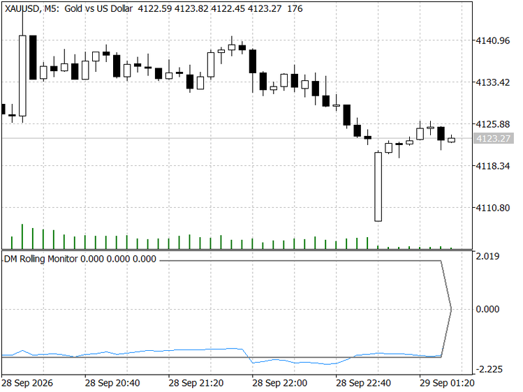
Fig. 3. DM_RollingMonitor running live on XAUUSD M5 - the rolling HLN-corrected DM statistic (blue) moves bar to bar against its two-tailed critical bands (gray, dotted), rather than sitting on a single flat value.

One trade-off worth knowing: the first calculation pass runs one ONNX inference per historical bar, so initial load over years of M5 data is noticeably slower than a typical indicator - expect a visible pause before the line appears. Live, incremental recalculation only touches the newest bar or two, so this is a one-time cost.

Edge cases and pitfalls

A few things will bite you if you don't handle them explicitly, so the implementation guards each one rather than letting it fail silently:

Loss series scale mismatch. If Model A and Model B output predictions in different units, the loss differential compares apples to oranges before the HAC step even runs. The implementation forces both forecasters into the same price-change units at the point of prediction, not at the loss calculation, so this can't sneak in silently.

Horizon collapse at h=1. At h=1 the HAC lag window is zero-length and the estimator reduces to plain sample variance - correct behavior, not a bug, as covered in Section 3.

Near-zero variance denominator. Nearly identical (or accidentally duplicated) forecasters can push the HAC variance toward zero and blow up the statistic through division. The code checks the denominator against a small epsilon and returns "no significant difference" directly rather than propagating a near-infinite statistic.

Insufficient sample size. Below roughly 30 observations the test loses its statistical footing, so the implementation returns an explicit "INSUFFICIENT_SAMPLE" verdict instead of a statistic that looks precise but isn't.

Common\Files, not MQL5\Files, for the ONNX model. The Strategy Tester runs each pass in its own private sandbox - a model placed only in the terminal folder loads live and fails in the Tester. OnnxCreate() uses ONNX_COMMON_FOLDER, so dm_forecaster.onnx and dm_manifest.json belong in the shared Common\Files\DMTest\ folder instead.

Indicator recompute cost. DM_RollingMonitor.mq5's first-load pass runs one ONNX inference per historical bar - real work on multi-year history, not a hang (see Section 8).

Cross-instrument comparisons. Reusing this test to compare one model's accuracy across instruments is mathematically possible but statistically riskier, since autocorrelation structure differs across volatility regimes and sessions. Treat it as a separate calibration exercise, not a drop-in reuse of the same settings.

Testing in the Strategy Tester

A verdict nobody acts on isn't worth much, so DM_Test_EA trades its own signal: on A_BETTER or B_BETTER it opens a position in that model's forecast direction at a fixed 0.01 lot with SL/TP at 1.5x/2x ATR, clamped to the broker's real min-lot/margin/stop-distance limits, staying flat on NO_SIGNIFICANT_DIFF - a genuine trade-count and drawdown result instead of a Journal-only statistic. Run it on visual mode with a fixed out-of-sample window and no re-fitting mid-run.

Setting	Value
Symbol/Timeframe	XAUUSD / M5
Forecast horizon (h)	1 bar
Loss function	Squared error
Rolling window	250 bars
Minimum sample size	30 bars
Significance level (alpha)	0.10, two-tailed
Dashboard refresh	Every 5 bars

Fig. 4 is a screenshot from an actual visual-mode run with this configuration - 48,047 M5 bars processed end to end with zero errors. Static and rolling DM/HLN point the same direction (both negative, both A_BETTER), though the statistics differ in magnitude (-3.566 static vs -2.085 rolling, since rolling only sees the trailing 250-bar window) - agreement in direction, not magnitude, is what you should expect from a placeholder model with no fitted edge going in.

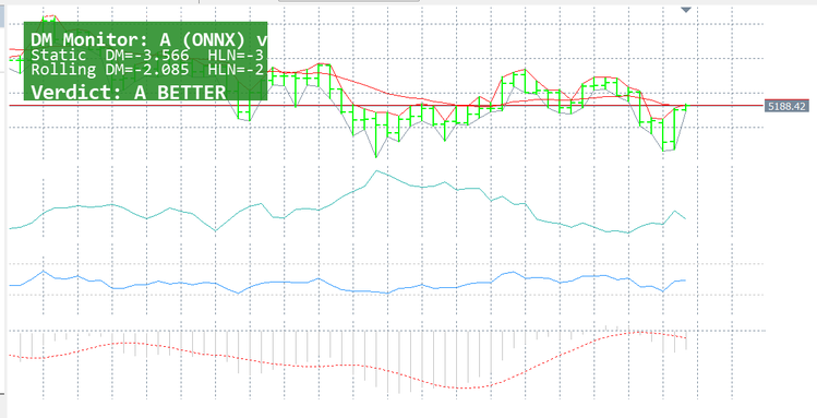
Fig. 4. DM_Test_EA running the configuration above in visual mode on XAUUSD M5 - the on-chart dashboard's static and rolling DM/HLN statistics and verdict, alongside the ATR(14), RSI(14), and MACD(12,26,9) inputs feeding the feature vector.

This run's full n/HLN/p triple wasn't captured in the Journal excerpt below, which is why the M5 row in the robustness table further down carries only the two DM figures, left blank rather than invented; the M15 and H1 rows, captured from the OnDeinit summary line, carry the complete figures and are the ones to treat as fully quantified evidence.

The Journal from a full end-to-end run with this configuration independently confirms the clean run. "final balance 10000.00" is the Tester's starting-deposit line, not an ending balance - the actual outcome is the XAUUSD M5 row in the trading-results table further down (Net Profit 86.84, ending balance roughly 10,086.84):

2026.01.01 00:00:00   DM_Test_EA: manifest loaded - h=1 window=250 min_n=30 loss=SQUARED
2026.01.01 00:00:00   ONNX: CPU selected
final balance 10000.00
XAUUSD,M5: 114028266 ticks, 48047 bars generated. Environment synchronized in 0:00:00.114. Test passed in 0:12:55.568 (including ti...
XAUUSD,M5: total time from login to stop testing 0:12:55.682 (including 0:00:00.114 for history data synchronization)
test Experts\DMTest\DM_Test_EA.ex5 on XAUUSD,M5 thread finished
shutdown finished

No OnInit failures, no ONNX load errors, no mid-run crashes - the run executed cleanly, but that says nothing about whether the statistical verdict or trading result are meaningful, which the rest of this section addresses with real numbers.

Multi-symbol, multi-timeframe robustness check

One clean M5 run proves the code doesn't crash, not that the edge is real. The EA ran across five symbol/timeframe combinations: three on XAUUSD, the instrument dm_forecaster.onnx's simulated training data stands in for (a placeholder model, not fitted on real XAUUSD history - see the file table at the end), and two on currency pairs it had never seen.

In-domain (XAUUSD, different timeframes) - whether the edge generalizes across horizons rather than being an artifact of one bar size:

Timeframe	Static n / DM / HLN / p	Rolling n / DM / HLN / p	Verdict (static / rolling)
M5*	- / -3.566 / - / -	- / -2.085 / - / -	A_BETTER / A_BETTER
M15	15230 / -4.678 / -4.678 / 0.0000	250 / -1.256 / -1.254 / 0.2111	A_BETTER / NO_SIGNIFICANT_DIFF
H1	3810 / -2.836 / -2.836 / 0.0046	250 / -0.743 / -0.741 / 0.4593	A_BETTER / NO_SIGNIFICANT_DIFF

*M5's n, HLN, and p weren't captured in this run's Journal excerpt - DM only, read from the dashboard screenshot. Treat the M15 and H1 rows as the fully quantified evidence.

Out-of-domain - the same EA and ONNX handle, unchanged, pointed at EURUSD and GBPUSD:

Symbol / Timeframe	Static n / DM / HLN / p	Rolling n / DM / HLN / p	Verdict (static / rolling)
EURUSD H1	4125 / 54.353 / 54.346 / 0.0000	250 / 12.022 / 11.998 / 0.0000	B_BETTER / B_BETTER
GBPUSD M5	49470 / 167.510 / 167.509 / 0.0000	250 / 21.688 / 21.644 / 0.0000	B_BETTER / B_BETTER

On XAUUSD, the static test finds a significant edge for Model A at every timeframe, weakening as the timeframe lengthens - p goes from effectively zero on M15 to 0.0046 on H1, consistent with smaller sample size, not a changing market. More tellingly, the rolling 250-bar window returns NO_SIGNIFICANT_DIFF on both M15 and H1: an edge real across nine months of M15 bars isn't visible in the most recent 250 of them, which is the rolling test doing its job, not a bug.

Read the out-of-domain numbers carefully. A genuine DM statistic on live market data is almost always 1–5; EURUSD H1 and GBPUSD M5 return 54 and 167, large enough that the honest reading is a scale mismatch, not a stronger result. Model A's ONNX model was trained offline, sized to XAUUSD's dollar-per-bar moves, and stays that scale regardless of instrument, while Model B's EMA slope recomputes live in each instrument's own units - pointed at EURUSD or GBPUSD, Model A's squared error dwarfs Model B's before either model says anything meaningful about direction. This is the cross-instrument pitfall from Section 9 in practice: B_BETTER at DM=54 or 167 means one forecaster is badly miscalibrated here, not that Model B genuinely out-forecasts Model A.

Taken together: a modest, timeframe-sensitive edge on the instrument this model was built for, and an immediate, correctly-flagged breakdown once either forecaster is pointed elsewhere. The same five runs also produced real trade counts, win rates, and drawdown.

Symbol / Timeframe	Trades	Net Profit	Profit Factor	Sharpe	Max DD
XAUUSD M5 (in-domain)	1083	86.84	1.01	0.47	4.91%
XAUUSD M15 (in-domain)	319	-717.54	0.81	-4.18	8.97%
XAUUSD H1 (in-domain)	121	221.91	1.11	1.42	3.58%
EURUSD H1 (out-of-domain)	332	-45.17	0.89	-1.31	0.88%
GBPUSD M5 (out-of-domain)	4273	-446.13	0.78	-5.00	4.52%

6,128 combined trades, and the DM pattern shows up in real money: both out-of-domain runs lose (negative Sharpe, Profit Factor under 1), while in-domain is genuinely mixed - M5 and H1 edge ahead, M15 loses outright. Worth flagging: 121 of 121 H1 trades and 315 of 319 M15 trades were short, a standing directional bias rather than context-sensitive skill - it paid off on H1's down-moves and lost on M15 for the same reason in reverse. No reliable edge, a reliably bad out-of-domain result, and an in-domain result driven more by a fixed short bias meeting favorable conditions than by adaptive forecasting.

Win rate alone doesn't say whether a run was profitable - that's profit factor above - but it does show whether the traded direction holds up as a coin-flip test. Fig. 5 plots the win rate from each of the five runs.

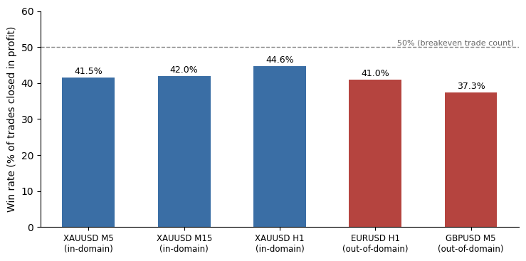
Fig. 5. Win rate by symbol/timeframe across the five real Strategy Tester runs. All five sit below 50%, in-domain and out-of-domain alike - the edge, where it exists at all, comes from win/loss size (profit factor), not from being right more often than wrong.

That's the value of a continuous rolling test over a one-off backtest statistic: a live read on whether to keep trusting Model A over Model B, not just which one won the last backtest. One caveat: the dashboard reruns this every g_dash_refresh bars over a 250-bar window that mostly overlaps the window five bars earlier, so successive p-values aren't independent draws - alpha=0.10 is the false-positive rate for one test, not for watching the dashboard flip color over weeks. Read a single rolling verdict as a snapshot, not an independent confirmation.

Reading the p-value like a trader, not a statistician

A rolling-window p-value of 0.03 does not imply future outperformance or profitability after costs - it only quantifies how unlikely the observed loss difference is under the null of equal expected loss, a statement about the current window's evidence, not a forecast.

So treat the dashboard's green/red/gray call as one input among several, not an automated trigger. A model can be significantly better with an effect too small to clear costs - watch mean_diff in the DMResult struct alongside the p-value, since a green verdict with a tiny mean_diff is a very different signal from one with a large one.

From pairwise to multi-model: extending toward a DM matrix

Everything here compares exactly two forecasters, the right scope for one article but rarely the end state of a real pipeline - most desks accumulate three, five, or a dozen candidates. The natural extension is a full pairwise DM matrix: run DM_RunTest() across every pair and assemble an N x N grid of statistics and p-values, which immediately shows clusters of indistinguishable models versus genuine standouts.

Two things change once you do this. Many pairwise tests reintroduce a multiple-comparisons problem - at 10% significance, testing 10 pairs produces roughly one false positive by chance alone, calling for a correction such as Benjamini-Hochberg FDR control. And the HAC lag structure should be re-validated per pair rather than assumed constant, since different architectures induce different autocorrelation on the same instrument. DMTest.mqh already takes any two error arrays and a horizon, with no assumption that there's only one comparison to run.

Limitations and what this doesn't prove

A few things this article and its numbers don't establish, stated plainly rather than glossed over:

Five runs is a robustness spot-check, not a robustness study. Three XAUUSD timeframes and two out-of-domain pairs isn't a large enough or randomized enough sample to claim the pattern generalizes beyond these five specific combinations.

Statistical significance isn't trading profitability. A_BETTER on XAUUSD M15 still lost money (Profit Factor 0.81) - a significantly lower forecast loss and a profitable trading system are different claims, and spread, slippage, and position sizing all sit outside what the test measures.

The fixed 1e-12 variance-denominator epsilon isn't scale-invariant. It was tuned to this article's raw price-change units on XAUUSD/EURUSD/GBPUSD; rescale it if you port this to a materially different price range, where it could be too loose or too tight.

DM_StudentQuantile()'s bisection range is hardcoded to [-100, 100]. Neither it nor DM_RunTest() validates that df or alpha stay inside where that bound is wide enough, so an extreme input from outside the manifest's normal values could silently return a quantile clipped at the boundary rather than erroring.

Verification against scipy is a handful of spot checks, not a test suite. dm_test_verify.py confirms agreement with scipy on the cases it was run against; it isn't automated and doesn't constitute regression coverage for the Student-t math or the DM statistic itself.

A clean Journal confirms the code ran, not that its output is correct. The 48,047-bar zero-error run earlier demonstrates operational stability, a real but separate claim from statistical or trading validity.

Conclusion

The Diebold-Mariano test isn't complicated math, but the details that make it trustworthy - HAC variance instead of naive sample variance, HLN small-sample correction instead of a normal-distribution shortcut - are exactly what most quick implementations skip. Skipping them doesn't make the test faster, it makes it wrong: significance where there's just shared volatility exposure, a statistic that assumes a sample size you don't have.

Wiring it into a live rolling dashboard turns it from a research curiosity into something you can check before changing allocation to a model. The five-run trading check is the other half: a statistically significant DM verdict and a genuinely profitable trade sequence aren't the same claim - in-domain results were mixed, out-of-domain lost money outright. The natural next step is feeding the rolling verdict into a capital-allocation layer, such as a Thompson Sampling or LinUCB selector shifting weight toward whichever forecaster currently wins, rather than reading the dashboard manually.

File	Type	Description
DMTest.mqh	Include	Core Diebold-Mariano math library: loss differential, Bartlett-kernel HAC variance, HLN correction, Student-t p-value, plus the shared feature builder and Model B forecast used identically by the EA and the indicator.
DM_Test_EA.mq5	Expert Advisor	Runs Model A (ONNX) and Model B (EMA-slope) forecasters live, maintains error histories, computes static and rolling DM tests, draws the CCanvas verdict dashboard, and trades the currently-winning model's direction with ATR-based SL/TP.
DM_RollingMonitor.mq5	Indicator	Subwindow visualization of a genuinely per-bar rolling HLN-corrected DM statistic with significance bands, recomputed via the same shared feature builder and a real ONNX forecast call.
dm_manifest.json	Config	Manifest driving horizon, loss type, rolling window, minimum sample size, and dashboard refresh - no hardcoded test parameters.
dm_test_verify.py	Python	Offline companion mirroring the MQL5 feature contract and DM math exactly, for automated consistency checks against EA-exported error logs.
dm_forecaster.onnx	Model	Placeholder 8-feature regressor (input [1,8], output [1,1]) matching the feature contract exactly, so the pipeline runs end-to-end out of the box. It's trained on simulated price data, not fitted to real XAUUSD history - retrain it on your own feature/return history from Section 5 before trusting any of its output.