
Overcoming The Limitation of Machine Learning (Part 1): Lack of Interoperable Metrics

Regrettably, the dangers of blindly following “best practices” silently corrupt other tools we rely on in our trading strategies, practitioners should not think this problem is unique to technical indicators.
In this series of articles, we shall explore critical problems that algorithmic traders are exposed to every day, by the very guidelines and practices intended to keep them safe when using machine learning models. Briefly, if the machine learning models being deployed on the MQL5 cloud every day remain aware of the facts presented in this discussion, ahead of the practitioners in charge, trouble is imminent. Investors may quickly find themselves exposed to more risk than they anticipated.
In all honesty, such problems are not emphasized enough, even in the world's leading books on statistical learning. The matter of our discussion is a simple truth that every practitioner in our community ought to know:
"It can be analytically proven, that the first derivative of Euclidean dispersion metrics such as RMSE, MAE or MSE can be solved by the mean of the target."
Practitioners already aware of this fact and its implications need not read on from this point.
However, it is for those practitioners who do not understand what this means, that I urgently need to reach through this article. In short, the regression metrics we use to build our models, are not suited for modelling asset returns.
This article will walk you through how this is happening, the dangers it presents to you, and what changes you can implement to start using this principle as a compass to filter down markets given a choice of hundreds of potential markets you could trade.
Practitioners who are desire deeper proof can find literature from Harvard University discussing the limitations of metrics such as RMSE. In particular, the Harvard paper offers an analytical proof that the mean of the sample minimizes RMSE. The reader can find the paper, linked, here.
Other institutions such as the Social Science Research Network, SSRN, maintain a journal of published and peer-reviewed papers from various domains, including a paper useful for our discussion, exploring alternative loss functions to substitute RMSE for asset pricing tasks. The paper, I have selected for the reader, reviews other papers in the field, and offers a summary of current literature before demonstrating a novel approach. This paper is readily available for the reader, here.
A Thought Experiment (Everyone Should Understand This)
Imagine you’re in a lottery-style competition. You and 99 other people are randomly selected to play for a $1,000,000 jackpot. The rules are simple; you must guess the heights of the other 99 participants. The winner is the person with the smallest total error across their 99 guesses.
Now, here’s the twist: for this example, imagine the average global human height is 1.1 meters. If you simply guess 1.1 meters for everyone, you might actually win the jackpot, even though every single prediction is technically wrong. Why? Because in noisy, uncertain environments, guessing the average tends to produce the smallest overall error.
The Trading Parallel
This thought experiment was intended to dramatize to the reader exactly how most machine learning models are selected for use in financial markets.
For instance, let’s say you’re building a model to forecast the S&P 500’s return. A model that always predicts the index’s historical average, roughly 7% annually, might actually outperform more complex models when judged by metrics like RMSE, MAE, or MSE. But here’s the trap: That model didn’t learn anything useful. It just clustered around the statistical mean. And worse, the metrics and validation procedures you trusted, rewarded it for doing so.
Beginner's Note: RMSE (Root Mean Square Error) is a “unit” used to judge the quality of machine learning models learning to forecast real valued targets.
It punishes large deviations but doesn't care why the model made the error, but remember, some of these deviations the model is punished for, were actually profit.
So a model that always predicts the average (even if it has zero market understanding) can look great on paper when judged with RMSE. This unfortunately allows us to create models that are mathematically sound, but practically useless.
What’s Really Going On
Financial data is noisy. We can’t observe key variables like true global supply/demand, investor sentiment, or institutional order book depth. So, to minimize error, your model will do the most statistically logical thing: predict the average.
And the reader must understand, that mathematically, it is sound practice. Predicting the mean minimizes most common regression errors. But trading isn’t about minimizing statistical error, it’s about making profitable decisions under uncertainty. And that distinction matters. In our community, such conduct is comparable to overfitting, but the statisticians who built these models, did not see things the same way we do.
It would be naive to think this problem is unique to regression models. In classification tasks, a model can minimize errors simply by always predicting the most common class in the training sample. And if the largest class in the training set, just so happens to correspond to the largest class in the entire population, I believe the practitioner can quickly see how a model can easily feign its skill.
Reward Hacking: When Models Win by Cheating
This phenomenon is called reward hacking: when a model achieves desirable performance levels, by learning undesirable behavior. In the case of trading, reward hacking results in practitioners choosing a model that appears skilled, but in reality the model is just playing a game of averages, a statistical house of cards. You think it’s learned something; but in reality it’s actually done the statistical equivalent of saying “everyone is 1.1 meters tall.” And RMSE accepts that, every time, without question.
Real Evidence
Now that our motivation is clear, let us depart from the use of allegory and instead consider real-world market data. Using the MetaTrader 5 Python API, I accessed 333 markets from my broker. We filtered for markets with at least four years of real-world historical data. This filter reduced our universe of markets down to 119.
We then built two models for each market:
- Control model: Always predicts the average 10-day return.
- Forecasting model: Attempts to learn and predict future returns.
Our Results
In 91.6% of the markets we tested, the control model won. That is to say, the model always predicting the historical average 10-day return produced lower error over 4 years, 91% of the time! As the practitioner will soon see, even when we tried deeper neural networks, the improvement was negligible.
Therefore, should the practitioner obey "best practices" of machine learning and always pick the model producing the lowest error, which remember, is the model always predicting the average return?
Beginner’s Note: This doesn’t mean machine learning can’t work for you. It means you need to be extremely cautious about how “good performance” should be defined in your trading context. If you fail to be careful, it would be reasonable for us to expect that you may unknowingly select a model being rewarded for predicting the average market return.
So What Now?
The takeaway is clear: the evaluation metrics we currently use—RMSE, MSE, MAE—aren’t designed for trading. They were born in statistics, medicine, and other natural sciences where predicting the mean makes sense. But in our algorithmic trading community, predicting the average return could be sometimes even worse than having no prediction at all, having no AI at all is sometimes safer. But AI without understanding is never safe!
We need evaluation frameworks that reward useful skill, not statistical cooperation metrics. We need metrics that understand profit and loss. Additionally, we need training protocols that penalize mean-hugging behavior, procedures that encourage the model to echo the values of our community while learning the realities of trading. And that’s what this series is focused on. A unique set of problems, that aren't being generated by the market directly. Rather, they are stemming from the very tools we wish to employ, and are seldom discussed in other articles, academic statistical learning books or even our own community discussions.
Practitioners need to be well versed with these facts, for their own safety. Regrettably, basic awareness of these limitations is not common knowledge that every member of our community has available at their fingertips. Everyday practitioners repeat very dangerous statistical practices without hesitation.
Getting Started
Let us see if there is any merit in what we have discussed so far. Load our standard libraries.
import pandas as pd
import numpy as np
import matplotlib.pyplot as plt
import MetaTrader5 as mt5
import multiprocessing as mp
Define how far into the future we wish to forecast.
HORIZON = 10Load the MetaTrader 5 terminal so we can fetch real-market data.
if(not mt5.initialize()):
   print("Failed to load MT5")
Get a comprehensive list of all available symbols.
symbols = mt5.symbols_get()
Just extract the names of the symbols.
symbols[0].name
symbol_names = []

for i in range(len(symbols)):
    symbol_names.append(symbols[i].name)
Now, get ready to see if we can outperform a model always predicting the mean.
from sklearn.linear_model import Ridge
from sklearn.model_selection import TimeSeriesSplit,cross_val_score
Create a time series validation splitter.
tscv = TimeSeriesSplit(n_splits=5,gap=HORIZON)We need a method, that will return our error levels when always predicting the average market return and our error levels when trying to predict the future market return.
def null_test(name):

    data_amount = 365 * 4

    f_data = pd.DataFrame(mt5.copy_rates_from_pos(name,mt5.TIMEFRAME_D1,0,data_amount))

    if(f_data.shape[0] < data_amount):
        print(f"{symbol_names[i]} did not have enough data!")
        return(None)

    f_data['time'] =pd.to_datetime(f_data['time'],unit='s')

    f_data['target'] = f_data['close'].shift(-HORIZON) - f_data['close']

    f_data.dropna(inplace=True)

    model = Ridge()

    res = []

    res.append(np.mean(np.abs(cross_val_score(model,f_data.loc[:,['open']] * 0,f_data['target'],cv=tscv))))
    res.append(np.mean(np.abs(cross_val_score(model,f_data.loc[:,['open','high','low','close']],f_data['target'],cv=tscv))))

    return(res)
Now we will perform the test across all the markets we have available.
res = pd.DataFrame(columns=['Mean Forecast','Direct Forecast'],index=symbol_names)

for i in range(len(symbol_names)):
    test_score = null_test(symbol_names[i])

    if(test_score is None):
        print(f"{symbol_names[i]} does not have enough data!")
        res.iloc[i,:] = [np.nan,np.nan]
        continue

    res.iloc[i,0] = test_score[0]
    res.iloc[i,1] = test_score[1]
    print(f"{i/len(symbol_names)}% complete.")

res['Score'] = ((res.iloc[:,1] / res.iloc[:,0]))
res.to_csv("Deriv Null Model Test.csv")
0.06606606606606606% complete.
0.06906906906906907% complete.
0.07207207207207207% complete.
...
GBPUSD RSI Trend Down Index did not have enough data!
GBPUSD RSI Trend Down Index does not have enough data!
From all the markets we had available, how many markets were we able to analyze?
#How many markets did we manage to investigate?
test = pd.read_csv("Null Model Test.csv")
print(f"{(test.dropna().shape[0] / test.shape[0]) * 100}% of Markets Were Evaluated")
35.73573573573574% of Markets Were Evaluated
We will now group our 119 markets based on a score associated with each market. The score will be the ratio of our error when predicting the market against our error when always predicting the average return. Scores smaller than 1 are impressive because it implies we outperformed a model always predicting the average return. Otherwise, scores greater than 1 validate our motivation for conducting this exercise in light of what we shared in the introduction of this article.
Beginner's Note: The scoring method we have briefly outlined is nothing new within machine learning. It is a metric commonly known as r-squared. It informs us how much of the variance in the target, we are explaining with our proposed model. We are not using the exact r-squared formula that you may be familiar with from your independent studies.
Let us first group all the markets where we obtained a score less than 1.
res.loc[res['Score'] < 1]
| Market Name | Mean Forecast | Direct Forecast | Score |
|---|---|---|---|
| AUDCAD | 0.022793 | 0.018566 | 0.814532 |
| EURCAD | 0.037192 | 0.027209 | 0.731587 |
| NZDCAD | 0.019124 | 0.015117 | 0.790466 |
| USDCNH | 0.125586 | 0.112814 | 0.898297 |
On what percentage of all the markets that we tested, did we outperform a model always predicting the average market return, over 4 years? Approximately 8%.
res.loc[res['Score'] < 1].shape[0] / res.shape[0]
0.08403361344537816
Therefore, that also implies that over 4 years, we could not outperform a model always predicting the average return for about 91.6% of all the markets we tested.
res.loc[res['Score'] > 1].shape[0] / res.shape[0]
0.9159663865546218
Now at this point some readers may be thinking that "The writer used simple linear models, if we took our time and built more flexible models, we could always outperform the model predicting the average return. This is nonsense". Which is partly true. Let us build a Deep Neural Network on the EURUSD market to outperform the model predicting the average market return.
First, we will need an MQL5 script to capture detailed market information about the EURUSD exchange rate. We will record the growths in each of the four price levels, and their growths regarding each other as well.
//+------------------------------------------------------------------+
//|                                                      ProjectName |
//|                                      Copyright 2020, CompanyName |
//|                                       http://www.companyname.net |
//+------------------------------------------------------------------+
#property copyright "Copyright 2024, MetaQuotes Ltd."
#property link      "https://www.mql5.com"
#property version   "1.00"
#property script_show_inputs

//+------------------------------------------------------------------+
//| System constants                                                 |
//+------------------------------------------------------------------+


//+------------------------------------------------------------------+
//| File name                                                        |
//+------------------------------------------------------------------+
string file_name = Symbol() + " IID Candlestick Recognition.csv";

//+------------------------------------------------------------------+
//| User inputs                                                      |
//+------------------------------------------------------------------+
input int size = 3000;
input int HORIZON = 10;

//+------------------------------------------------------------------+
//| Our script execution                                             |
//+------------------------------------------------------------------+
void OnStart()
  {

//---Write to file
   int file_handle=FileOpen(file_name,FILE_WRITE|FILE_ANSI|FILE_CSV,",");

   for(int i=size;i>=1;i--)
     {
      if(i == size)
        {
         FileWrite(file_handle,"Time","Open","High","Low","Close","Delta Open","Delta High","Delta Low","Delta Close","O - H","O - L","O - C","H - L","H - C","L - C");
        }

      else
        {
         FileWrite(file_handle,
                   iTime(_Symbol,PERIOD_CURRENT,i),
                   iOpen(_Symbol,PERIOD_CURRENT,i),
                   iHigh(_Symbol,PERIOD_CURRENT,i),
                   iLow(_Symbol,PERIOD_CURRENT,i),
                   iClose(_Symbol,PERIOD_CURRENT,i),
                   iOpen(_Symbol,PERIOD_CURRENT,i)  - iOpen(_Symbol,PERIOD_CURRENT,i + HORIZON),
                   iHigh(_Symbol,PERIOD_CURRENT,i)  - iHigh(_Symbol,PERIOD_CURRENT,i + HORIZON),
                   iLow(_Symbol,PERIOD_CURRENT,i)   - iLow(_Symbol,PERIOD_CURRENT,i + HORIZON),
                   iClose(_Symbol,PERIOD_CURRENT,i) - iClose(_Symbol,PERIOD_CURRENT,i + HORIZON),
                   iOpen(_Symbol,PERIOD_CURRENT,i)  - iHigh(_Symbol,PERIOD_CURRENT,i),
                   iOpen(_Symbol,PERIOD_CURRENT,i)  - iLow(_Symbol,PERIOD_CURRENT,i),
                   iOpen(_Symbol,PERIOD_CURRENT,i)  - iClose(_Symbol,PERIOD_CURRENT,i),
                   iHigh(_Symbol,PERIOD_CURRENT,i)  - iLow(_Symbol,PERIOD_CURRENT,i),
                   iHigh(_Symbol,PERIOD_CURRENT,i)  - iClose(_Symbol,PERIOD_CURRENT,i),
                   iLow(_Symbol,PERIOD_CURRENT,i)   - iClose(_Symbol,PERIOD_CURRENT,i)
                  );
        }
     }
//--- Close the file
   FileClose(file_handle);
  }

//+------------------------------------------------------------------+

//+------------------------------------------------------------------+
//| Undefine system constants                                        |
//+------------------------------------------------------------------+
#undef HORIZON
Now drag and drop your script onto the chart to fetch historical data about the market, and then we can get started.
#Read in market data
HORIZON = 10
data = pd.read_csv('EURUSD IID Candlestick Recognition.csv')

#Label the data
data['Null'] = 0
data['Target'] = data['Close'].shift(-HORIZON) - data['Close']

#Drop the last HORIZON rows of data
data = data.iloc[:-HORIZON,:]

data
Readers who think deep neural networks and sophisticated models will solve the problem of outperforming a model predicting the average market return, will be shocked to read what follows in the rest of this article.
I encourage you to repeat this experiment with your broker, before deploying your models with your capital. Let us now load the scikit learn tools to compare how well our deep neural network is performing against our simple linear model.
#Load our models
from sklearn.neural_network import MLPRegressor
from sklearn.linear_model       import Ridge
from sklearn.model_selection import TimeSeriesSplit,train_test_split,cross_val_score
Split the data.
#Split the data into half
train,test = train_test_split(data,test_size=0.5,shuffle=False)
Create a time series validation object.
#Create a time series validation object
tscv = TimeSeriesSplit(n_splits=5,gap=HORIZON)
Fit the model always predicting the average market return. The error caused by always predicting the mean is named the "total sum of squares". The TSS is a critical error benchmark in machine learning, it tells us which way is North.
#Fit the model predicting the mean on the train set
null_model = Ridge()

null_model.fit(train[['Null']],train['Target'])

tss = np.mean(np.abs(cross_val_score(null_model,test[['Null']],test['Target'],cv=tscv,scoring='neg_mean_absolute_error')))

tss
np.float64(0.011172426520738554)
Define our inputs and target.
X = data.iloc[:,4:-2].columns
y = 'Target'
Fit your deep neural network. I encourage the reader to feel welcome to adjust this neural network however they see fit to see if they have what it takes, to outperform the mean.
#Let us now try to outperform the null model
model = MLPRegressor(activation='logistic',solver='lbfgs',random_state=0,shuffle=False,hidden_layer_sizes=(len(X),200,50),max_iter=1000,early_stopping=False)

model.fit(train.loc[:,X],train['Target'])

rss = np.mean(np.abs(cross_val_score(model,test.loc[:,X],test['Target'],cv=tscv,scoring='neg_mean_absolute_error')))

print(f"Test Passed: {rss < tss} || New R-Squared Metric {rss/tss}")

res = []

res.append(rss)
res.append(tss)

sns.barplot(res,color='black')
plt.axhline(tss,color='red',linestyle=':')
plt.grid()
plt.ylabel("RMSE")
plt.xticks([0,1],['Deep Neural Network','Null Model'])
plt.title("Our Deep Neural Network vs The Null Model")
plt.show()
After a lot of configuring, adjustments and optimizing, I was able to defeat the model predicting the average return, using a deep neural network. However, let us take a closer look at what's happening here.
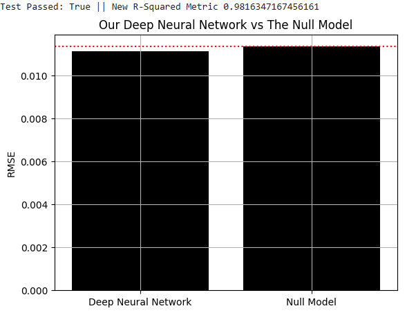
Fig 1: Outperforming a model predicting the average market return is materially challenging
Let us visualize the improvements our Deep Neural Network is making. First, I will set up a grid for us to assess the distribution of the market's returns in the test set, and the distributions of the returns our model predicted. Store the returns the model predicts for the test set.
predictions = model.predict(test.loc[:,X])
We will start by first marking the average market return we observed in the training set as the red dotted line in the middle of the graph.
plt.title("Visualizing Our Improvements")
plt.plot()
plt.grid()
plt.xlabel("Return")
plt.axvline(train['Target'].mean(),color='red',linestyle=':')
legend = ['Train Mean']
plt.legend(legend)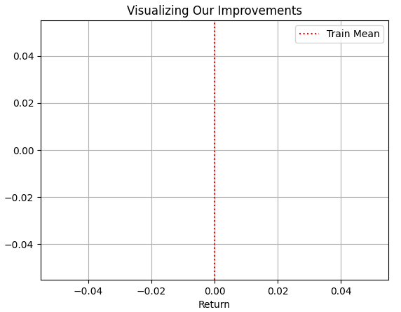
Fig 2: Visualizing the average market return from the training set
Now, let us overlay the model's prediction for the test set, on top of the average return from the train set. As the reader can see, the model's predictions are spread around the mean of the training set. However, the problem becomes clear, when we finally overlay the true distribution the market followed as a black graph underneath.
plt.title("Visualizing Our Improvements")
plt.plot()
plt.grid()
plt.xlabel("Return")
plt.axvline(train['Target'].mean(),color='red',linestyle=':')
sns.histplot(predictions,color='blue')
legend = ['Train Mean','Model Predictions']
plt.legend(legend)
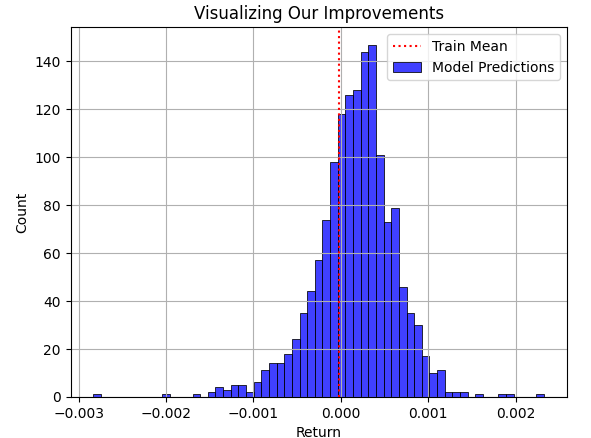
Fig 3: Visualizing our model's predictions regarding the average return the model observed in the training set
The blue region of predictions being made by our model appeared reasonable in Fig 3, but when we finally consider the true distribution the market followed in Fig 4, it becomes apparent that this model is not sound for the task at hand. The model is failing to capture the width of the market's true distribution, where some of the largest profits and losses are hiding from our model's awareness. Regrettably, RMSE will frequently point practitioners to such models, if the metric of RMSE is not carefully understood, respected and interpreted by the practitioner in charge. Using such a model in real trading would be catastrophic for your live trading experience.
plt.title("Visualizing Our Improvements")
plt.plot()
plt.grid()
plt.xlabel("Return")
plt.axvline(train['Target'].mean(),color='red',linestyle=':')
sns.histplot(test['Target'],color='black')
sns.histplot(predictions,color='blue')

legend = ['Train Mean','Test Distribution','Model Prediction']
plt.legend(legend)
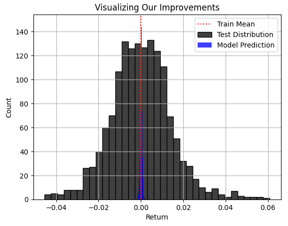
Fig 4: Visualizing the distribution of our models' predictions regarding the true distribution of the market
Our Proposed Solution
At this point, we demonstrated to the reader that metrics such as RMSE can easily be optimized by always predicting the average market return, and we demonstrated why this is unattractive because RMSE could frequently report to us that such a useless model, is the best we can do. We expressed that, clearly, there is a need for procedures and new techniques that explicitly:
- Test real-world market understanding.
- Understand the difference between profit and loss.
- Discourage mean hugging behavior.
I'd like to propose a unique model architecture that could be a possible candidate solution the reader can consider. I refer to the strategy as "Dynamic Regime Switching Models" or DRS for short. In a separate discussion on high probability setups, we observed that modelling the profit/loss generated by a trading strategy may be easier than trying to forecast the market directly. Readers who have not yet read that article, can find that article linked, here.
We shall now proceed to exploit that observation in a manner that is interesting. We shall build two identical models, to simulate opposing versions of one trading strategy. One model will always assume the market is in a trend following state, while the last always assumes the market is in a mean reverting state. Each model will be trained separately and has no awareness, or means to coordinate its predictions with the other model.
The reader should recall that the Efficient Market Hypothesis teaches investors that buying and selling the same volumes of the same asset will leave the investor perfectly hedged, and if both positions are opened and closed simultaneously, the total profit is 0, not including any transaction fees. Therefore, we should expect that our models should always agree with this fact. In fact, we can test if our models agree with this truth, models that do not agree with this truth, have no true market understanding.
Therefore, we can substitute the need to rely on metrics such as RMSE by rather testing if our DVM model demonstrates an understanding of this principle that builds market structure. Here is where our test for real-world market understanding comes to play. If both our models truly understand the realities of trading, then the sum of their forecasts should always total 0, at all times. We will fit our models on the training set, and then test them out-of-sample, to see if the model's predictions always sum to 0 even when the models are under-stressed.
Recall that the predictions of the models are not being coordinated in any way, shape or form. The models are trained separately, and have no awareness of each other. Therefore, if the models are not "hacking" desirable error metrics but truly learning the underlying structure of the market, then they will prove that they have arrived at their predictions through ethical conduct if both the model's predictions sum to 0.
Only one of these models can expect positive reward at any instance in time. If the sum of our model's predictions is not 0, then the models may have unintentionally learned a directional bias that violates the efficient market hypothesis. Otherwise, in the best-case scenario, we can dynamically alternate between these 2 market states with a level of confidence we're not familiar with in the past. Only one model should expect a positive reward at any single moment, and our trading philosophy is that we believe that model corresponds to the hidden state the market is currently in. And this could potentially be worth more to us, than low RMSE readings.
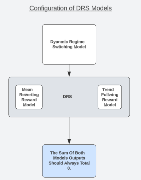
Fig 5: Understanding the general architecture of our DRS models
Fetching Data From Our Terminal
Our data should be as detailed as possible for the best results. Therefore, we are keeping track of the current values of our technical indicators and price levels, as well as the growth that has been occurring in these market dynamics at the same time.
//+------------------------------------------------------------------+
//|                                                      ProjectName |
//|                                      Copyright 2020, CompanyName |
//|                                       http://www.companyname.net |
//+------------------------------------------------------------------+
#property copyright "Copyright 2024, MetaQuotes Ltd."
#property link      "https://www.mql5.com"
#property version   "1.00"
#property script_show_inputs

//--- Define our moving average indicator
#define MA_PERIOD 5                //--- Moving Average Period
#define MA_TYPE   MODE_SMA          //--- Type of moving average we have
#define HORIZON 10

//--- Our handlers for our indicators
int ma_handle;

//--- Data structures to store the readings from our indicators
double ma_reading[];

//--- File name
string file_name = Symbol() + " DRS Modelling.csv";

//--- Amount of data requested
input int size = 3000;

//+------------------------------------------------------------------+
//| Our script execution                                             |
//+------------------------------------------------------------------+
void OnStart()
  {
  int fetch = size + (HORIZON * 2);
//---Setup our technical indicators
   ma_handle = iMA(_Symbol,PERIOD_CURRENT,MA_PERIOD,0,MA_TYPE,PRICE_CLOSE);

//---Set the values as series
   CopyBuffer(ma_handle,0,0,fetch,ma_reading);
   ArraySetAsSeries(ma_reading,true);

//---Write to file
   int file_handle=FileOpen(file_name,FILE_WRITE|FILE_ANSI|FILE_CSV,",");

   for(int i=size;i>=1;i--)
     {
      if(i == size)
        {
         FileWrite(file_handle,"Time","Open","High","Low","Close","Delta O","Delta H","Delta Low","Delta Close","SMA 5","Delta SMA 5");
        }

      else
        {
         FileWrite(file_handle,
                   iTime(_Symbol,PERIOD_CURRENT,i),
                   iOpen(_Symbol,PERIOD_CURRENT,i),
                   iHigh(_Symbol,PERIOD_CURRENT,i),
                   iLow(_Symbol,PERIOD_CURRENT,i),
                   iClose(_Symbol,PERIOD_CURRENT,i),
                   iOpen(_Symbol,PERIOD_CURRENT,i)   - iOpen(_Symbol,PERIOD_CURRENT,(i + HORIZON)),
                   iHigh(_Symbol,PERIOD_CURRENT,i)   - iHigh(_Symbol,PERIOD_CURRENT,(i + HORIZON)),
                   iLow(_Symbol,PERIOD_CURRENT,i)    - iLow(_Symbol,PERIOD_CURRENT,(i + HORIZON)),
                   iClose(_Symbol,PERIOD_CURRENT,i)  - iClose(_Symbol,PERIOD_CURRENT,(i + HORIZON)),
                   ma_reading[i],
                   ma_reading[i] - ma_reading[(i + HORIZON)]
                   );
        }
     }
//--- Close the file
   FileClose(file_handle);
  }
//+------------------------------------------------------------------+
Getting Started
To get the ball rolling, we will first import our standard libraries.
#Load our libraries
import pandas as pd
import numpy as np
import matplotlib.pyplot as plt
import seaborn as sns
Now we can read in the data we wrote out to CSV earlier.
#Read in the data
data = pd.read_csv("/content/drive/MyDrive/Colab Data/Financial Data/FX/EUR USD/DRS Modelling/EURUSD DRS Modelling.csv")
data
When we built our MQL5 script, we were forecasting 10 steps into the future. We must maintain that.
#Recall that in our MQL5 Script our forecast horizon was 10
HORIZON = 10

#Calculate the returns generated by the market
data['Return'] = data['Close'].shift(-HORIZON) - data['Close']

#Drop the last horizon rows
data = data.iloc[:-HORIZON,:]
Now label the data. Recall that we will have 2 labels, one always assuming the market is going to continue in a trend, and the other label always assumes the market is stuck in mean-reverting behavior.
#Now let us define the signals being generated by the moving average, in the DRS framework there are always at least n signals depending on the n states the market could be in
#Our simple DRS model assumes only 2 states
#First we will define the actions you should take assuming the market is in a trending state
#Therefore if price crosses above the moving average, buy. Otherwise, sell.
data['Trend Action'] = 0

data.loc[data['Close'] > data['SMA 5'], 'Trend Action'] = 1
data.loc[data['Close'] < data['SMA 5'], 'Trend Action'] = -1

#Now calculate the returns generated by the strategy
data['Trend Profit'] = data['Trend Action'] * data['Return']
After labelling the trend following actions, insert the mean reverting actions.
#Now we will repeat the procedure assuming the market was mean reverting
data['Mean Reverting Action'] = 0

data.loc[data['Close'] > data['SMA 5'], 'Mean Reverting Action'] = -1
data.loc[data['Close'] < data['SMA 5'], 'Mean Reverting Action'] = 1

#Now calculate the returns generated by the strategy
data['Mean Reverting Profit'] = data['Mean Reverting Action'] * data['Return']
By labelling the data this way, our hopes are that the computer will pick up the conditions in which each strategy loses money and when to listen to each strategy. If we plot the cumulative target value, we can clearly see that over the selected time period in our data, the EURUSD market spent more time demonstrating mean reverting behavior than trend following. However, note that both lines have sudden shocks in them. I believe these shocks, may correspond to sudden regime changes in the market.
#If we plot our cumulative profit sums, we can see the profit and losses aren't evenly distributed between the two states
plt.plot(data['Trend Profit'].cumsum(),color='black')
plt.plot(data['Mean Reverting Profit'].cumsum(),color='red')

#The mean reverting strategy appears to have been making outsized profits with respect to the trending stratetefgy
#However, closer inspection reveals, that both strategies are profitable, but never at the same time!
#The profit profiles of both strategies show abrupt shocks, when the opposite strategy become more profitable.
plt.legend(['Trend Profit','Mean Reverting Profit'])
plt.xlabel('Time')
plt.ylabel('Profit/Loss')
plt.title('A DRS Model Visualizes The Market As Being in 2 Possible States')
plt.grid()
plt.axhline(0,color='black',linestyle=':')
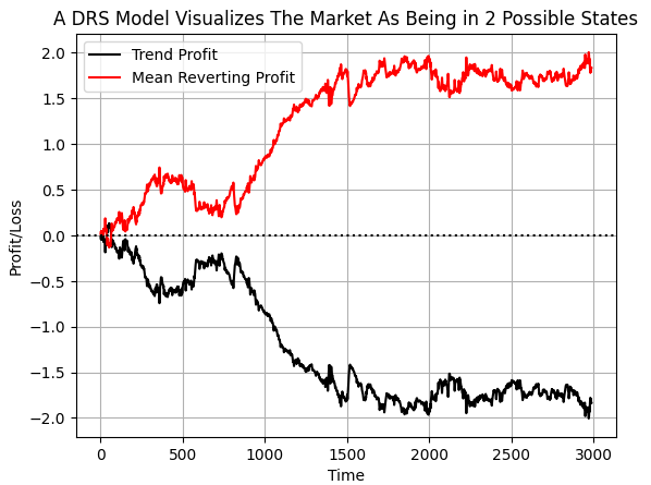
Fig 6:Visualizing the distribution of profit across 2 opposing strategies
Define your inputs and target.
#Let's define the inputs and target
X = data.iloc[:,1:-5].columns
y = ['Trend Profit','Mean Reverting Profit']
Select our tools for modelling the market.
#Import the modelling tools
from sklearn.model_selection import train_test_split,TimeSeriesSplit
from sklearn.ensemble import RandomForestRegressor
Split the data twice. So that we have a training set, validation set, and final test set.
#Split the data
train , test = train_test_split(data,test_size=0.5,shuffle=False)

f_train , f_validation = train_test_split(train,test_size=0.5,shuffle=False)
Prepare our 2 models now. Recall that both models will give us a Dual-View of the world, but they should not be coordinated in any fashion.
#The trend model
trend_model = RandomForestRegressor()

#The mean reverting model
mean_model = RandomForestRegressor()
Fit our models.
trend_model.fit(f_train.loc[:,X],f_train.loc[:,y[0]])
mean_model.fit(f_train.loc[:,X],f_train.loc[:,y[1]])
Testing the validity of our models. We will record both model's predictions of what values their targets will take in the test set. Recall, the models are not learning the same target. Each model independently learned its own target, and worked to reduce its error independent of the other model.
pred_1 = trend_model.predict(f_validation.loc[:,X])
pred_2 = mean_model.predict(f_validation.loc[:,X])
The contents of the validation set are out of sample for our models. We are essentially stress testing the models using data they have not seen before, to observe if our models will behave in an ethical manner under material stress.
Our test is performed on the sum of both model's predictions. If the maximum value of the sum of the model's predictions equals 0.0, then our model has passed our test. Because our model essentially agrees with the efficient market hypothesis that by following both models at the same time, the investor will make nothing. We intend to follow only 1 model at a time. Therefore, we will be dynamically switching between regimes. This is to say, our strategy, has the ability to change strategy without human intervention.
test_result = pred_1 + pred_2

print(f" Test Passed: {np.linalg.norm(test_result,ord=2) == 0.0}")
The numpy package contains many useful libraries, such as the linear algebra package we used above. The norm function we called simply returns the total sum of a vector's contents, or the largest value in a vector, depending on how the method is called. This is logically the same as manually checking the contents of the array for yourself, to ensure all the numbers in the array are 0. Note I have truncated the outputs of the array, but the reader can rest assured, they were all 0.
array([0., 0., 0., 0., 0., 0., 0., 0., 0., 0., 0., 0., 0., 0., 0., 0., 0.,
0., 0., 0., 0., 0., 0., 0., 0., 0., 0., 0., 0., 0., 0., 0., 0., 0.,
When we plot the actual profit made the trend following strategy and compare it to the predictions made by the trend following model, we realize that withholding a few massive swings in profitability such as during the 600 and 700-day interval, when the ERUUSD market swung with significant volatility, our model was able to keep up with the other normally sized profits.
plt.plot(f_validation.loc[:,y[0]],color='black')
plt.plot(pred_1,color='red',linestyle=':')
plt.legend(['Actual Profit','Predicted Profit'])
plt.grid()
plt.ylabel('Loss / Profit')
plt.xlabel('Out Of Sample Days')
plt.title('Visualizing Our Model Performance Out Of Sample on the EURUSD 10 Day Return')
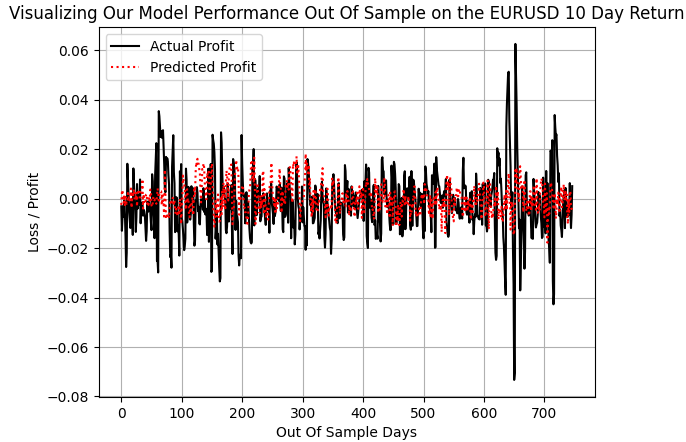
Fig 7: Our DRS model failed to capture the true volatility of the market
We are now ready to export our machine learning models to ONNX format, and begin guiding our trading applications in new directions. ONNX stands for Open Neural Network Exchange, and it allows us to build and deploy machine learning models through a set of widely adopted API's. This widespread adoption, allows different programming languages to work with the same ONNX model. And recall, each ONNX model, is just a representation of your machine learning model. If you do not have skl2onnx and ONNX libraries already installed, start by installing them.
!pip install skl2onnx onnx
Now load the libraries we need to export.
import onnx
from skl2onnx import convert_sklearn
from skl2onnx.common.data_types import FloatTensorType
Define the I/O shape of your ONNX models.
eurusd_drs_shape = [("float_input",FloatTensorType([1,len(X)]))]
eurusd_drs_output_shape = [("float_output",FloatTensorType([1,1]))]
Prepare ONNX prototypes of your DRS model.
trend_drs_model_proto = convert_sklearn(trend_model,initial_types=eurusd_drs_shape,final_types=eurusd_drs_output_shape,target_opset=12)
mean_drs_model_proto = convert_sklearn(mean_model,initial_types=eurusd_drs_shape,final_types=eurusd_drs_output_shape,target_opset=12)
Save the models.
onnx.save(trend_drs_model_proto,"EURUSD RF D1 T LBFGSB DRS.onnx")
onnx.save(mean_drs_model_proto,"EURUSD RF D1 M LBFGSB DRS.onnx")
Congratulations, you have built your first DRS model architecture. Let us now get ready to back test the models, and see if they make a difference, and whether we were able to meaningfully substitute the RMSE from our design process.
Getting Started in MQL5
To get started, first we will define system constants that are important for our trading activities.
//+------------------------------------------------------------------+
//|                                                   EURUSD DRS.mq5 |
//|                                  Copyright 2024, MetaQuotes Ltd. |
//|                                             https://www.mql5.com |
//+------------------------------------------------------------------+
#property copyright "Copyright 2024, MetaQuotes Ltd."
#property link      "https://www.mql5.com"
#property version   "1.00"

//+------------------------------------------------------------------+
//| System constants                                                 |
//+------------------------------------------------------------------+
#define HORIZON 10
#define MA_PERIOD 5
#define MA_SHIFT 0
#define MA_MODE MODE_SMA
#define TRADING_VOLUME SymbolInfoDouble(Symbol(),SYMBOL_VOLUME_MIN)
Now we can load our system resources.
//+------------------------------------------------------------------+
//| System dependencies                                              |
//+------------------------------------------------------------------+
#resource "\\Files\\DRS\\EURUSD RF D1 T DRS.onnx" as uchar onnx_proto[]   //Our Trend Model
#resource "\\Files\\DRS\\EURUSD RF D1 M DRS.onnx" as uchar onnx_proto_2[] //Our Mean Reverting Mode
Load the trade library.
//+------------------------------------------------------------------+
//| System libraries                                                 |
//+------------------------------------------------------------------+
#include <Trade/Trade.mqh>
CTrade Trade;
We will also need variables for our technical indicators.
//+------------------------------------------------------------------+
//| Technical Indicators                                             |
//+------------------------------------------------------------------+
int    ma_o_handle,ma_c_handle,atr_handle;
double ma_o[],ma_c[],atr[];
double bid,ask;
int    holding_period;
Specify global variables.
//+------------------------------------------------------------------+
//| Global variables                                                 |
//+------------------------------------------------------------------+
long onnx_model,onnx_model_2;
When our application is initially loaded, we will call a method responsible for loading our technical indicators and ONNX models.
//+------------------------------------------------------------------+
//| Expert initialization function                                   |
//+------------------------------------------------------------------+
int OnInit()
  {
//---
   if(!setup()) return(INIT_FAILED);
//---
   return(INIT_SUCCEEDED);
  }
If we aren't using the application, let us clean up the resources we no longer need.
//+------------------------------------------------------------------+
//| Expert deinitialization function                                 |
//+------------------------------------------------------------------+
void OnDeinit(const int reason)
  {
//---
   release();
  }
Finally, when we receive updated price levels, we will either look for a trading opportunity or manage the open positions we have.
//+------------------------------------------------------------------+
//| Expert tick function                                             |
//+------------------------------------------------------------------+
void OnTick()
  {
//---
   static datetime time_stamp;
   datetime current_time = iTime(Symbol(),PERIOD_D1,0);

   if(time_stamp != current_time)
     {
      time_stamp = current_time;
      update_variables();

      if(PositionsTotal() == 0)
        {
         find_setup();
        }

      else
         if(PositionsTotal() > 0)
           {
            manage_setup();
           }
     }
  }
//+------------------------------------------------------------------+
This is the implementation of the function we wrote to set up the entire system.
//+------------------------------------------------------------------+
//| Attempt To Setup Our System Variables                            |
//+------------------------------------------------------------------+
bool setup(void)
  {

   atr_handle = iATR(Symbol(),PERIOD_CURRENT,14);
   ma_c_handle = iMA(Symbol(),PERIOD_CURRENT,MA_PERIOD,MA_SHIFT,MA_MODE,PRICE_CLOSE);
   ma_o_handle = iMA(Symbol(),PERIOD_CURRENT,MA_PERIOD,MA_SHIFT,MA_MODE,PRICE_OPEN);
   holding_period = 0;

   onnx_model = OnnxCreateFromBuffer(onnx_proto,ONNX_DEFAULT);
   onnx_model_2 = OnnxCreateFromBuffer(onnx_proto_2,ONNX_DEFAULT);

   if(onnx_model == INVALID_HANDLE)
     {
      Comment("Failed to load Trend DRS model");
      return(false);
     }

   if(onnx_model_2 == INVALID_HANDLE)
     {
      Comment("Failed to load Mean Reverting DRS model");
      return(false);
     }


   ulong input_shape[] = {1,10};
   ulong output_shape[] = {1,1};

   if(!OnnxSetInputShape(onnx_model,0,input_shape))
     {
      Comment("Failed to set Trend DRS Model input shape");
      return(false);
     }

   if(!OnnxSetInputShape(onnx_model_2,0,input_shape))
     {
      Comment("Failed to set Mean Reverting DRS Model input shape");
      return(false);
     }

   if(!OnnxSetOutputShape(onnx_model,0,output_shape))
     {
      Comment("Failed to set Trend DRS Model output shape");
      return(false);
     }

   if(!OnnxSetOutputShape(onnx_model_2,0,output_shape))
     {
      Comment("Failed to set Mean Reverting DRS Model output shape");
      return(false);
     }
   return(true);
  }
When we deinitialize the system, we will manually release the indicators and ONNX models we aren't using anymore.
//+------------------------------------------------------------------+
//| Free up system resources                                         |
//+------------------------------------------------------------------+
void release(void)
  {
   IndicatorRelease(ma_c_handle);
   IndicatorRelease(ma_o_handle);
   OnnxRelease(onnx_model);
   OnnxRelease(onnx_model_2);
  }
Update the system variables whenever we have new price information.
//+------------------------------------------------------------------+
//| Update our system variables                                      |
//+------------------------------------------------------------------+
void update_variables(void)
  {
   bid = SymbolInfoDouble(Symbol(),SYMBOL_BID);
   ask = SymbolInfoDouble(Symbol(),SYMBOL_ASK);
   CopyBuffer(ma_c_handle,0,1,(HORIZON*2),ma_c);
   CopyBuffer(ma_o_handle,0,1,(HORIZON*2),ma_o);
   CopyBuffer(atr_handle,0,0,1,atr);
   ArraySetAsSeries(ma_c,true);
   ArraySetAsSeries(ma_o,true);
  }
Manage open trades, by essentially counting down to our 10-day return.
//+------------------------------------------------------------------+
//| Manage The Trade We Have Open                                    |
//+------------------------------------------------------------------+
void manage_setup(void)
  {
   if((PositionsTotal() > 0) && (holding_period < (HORIZON-1)))
      holding_period +=1;

   else
      if((PositionsTotal() > 0) && (holding_period == (HORIZON - 1)))
         Trade.PositionClose(Symbol());
  }
Find a trading setup by fetching detailed information about the current market state, and feeding it to our model. Our strategy relies on using moving averages as indicators of investor sentiment. When the moving averages give short signals, we will assume most investors want to go short, but we believe that the majority tends to be wrong in the FX market
//+------------------------------------------------------------------+
//| Find A Trading Oppurtunity For Our Strategy                      |
//+------------------------------------------------------------------+
void find_setup(void)
  {
   vectorf model_inputs   = vectorf::Zeros(10);
   vectorf model_outputs  = vectorf::Zeros(1);
   vectorf model_2_outputs  = vectorf::Zeros(1);
   holding_period = 0;
   int i = 0;

   model_inputs[0] = (float) iOpen(Symbol(),PERIOD_CURRENT,0);
   model_inputs[1] = (float) iHigh(Symbol(),PERIOD_CURRENT,0);
   model_inputs[2] = (float) iLow(Symbol(),PERIOD_CURRENT,0);
   model_inputs[3] = (float) iClose(Symbol(),PERIOD_CURRENT,0);
   model_inputs[4] = (float)(iOpen(Symbol(),PERIOD_CURRENT,0) - iOpen(Symbol(),PERIOD_CURRENT,HORIZON));
   model_inputs[5] = (float)(iHigh(Symbol(),PERIOD_CURRENT,0) - iHigh(Symbol(),PERIOD_CURRENT,HORIZON));
   model_inputs[6] = (float)(iLow(Symbol(),PERIOD_CURRENT,0) - iLow(Symbol(),PERIOD_CURRENT,HORIZON));
   model_inputs[7] = (float)(iClose(Symbol(),PERIOD_CURRENT,0) - iClose(Symbol(),PERIOD_CURRENT,HORIZON));
   model_inputs[8] = (float) ma_c[0];
   model_inputs[9] = (float)(ma_c[0] - ma_c[HORIZON]);

   if(!OnnxRun(onnx_model,ONNX_DEFAULT,model_inputs,model_outputs))
     {
      Comment("Failed to run the ONNX model correctly.");
     }

   if(!OnnxRun(onnx_model_2,ONNX_DEFAULT,model_inputs,model_2_outputs))
     {
      Comment("Failed to run the ONNX model correctly.");
     }

   if(model_outputs[0] > 0)
     {
      if(ma_c[0] < ma_o[0])
        {
         if(iClose(Symbol(),PERIOD_CURRENT,0) > ma_c[0])
            Trade.Buy(TRADING_VOLUME,Symbol(),ask,0,0,"");
        }

      else
         if(ma_c[0] > ma_o[0])
           {
            if(iClose(Symbol(),PERIOD_CURRENT,0) < ma_c[0])
               Trade.Sell(TRADING_VOLUME,Symbol(),bid,0,0,"");
           }
     }

   else
      if(model_2_outputs[0] > 0)
        {
         if(ma_c[0] < ma_o[0])
           {
            if(iClose(Symbol(),PERIOD_CURRENT,0) < ma_c[0])
               Trade.Buy(TRADING_VOLUME,Symbol(),ask,0,0,"");
           }

         if(ma_c[0] > ma_o[0])
           {
            if(iClose(Symbol(),PERIOD_CURRENT,0) > ma_c[0])
               Trade.Sell(TRADING_VOLUME,Symbol(),bid,0,0,"");
           }
        }

   Comment("0: ",model_outputs[0],"1: ",model_2_outputs[0]);
  }
Undefine system constants.
//+------------------------------------------------------------------+
//| Undefine system constants                                        |
//+------------------------------------------------------------------+
#undef HORIZON
#undef MA_MODE
#undef MA_PERIOD
#undef MA_SHIFT
#undef TRADING_VOLUME
//+------------------------------------------------------------------+
First, we shall select our back test dates. Recall that we always pick dates that lie beyond the model's training set to get a reliable idea of how well the model may perform in the future.
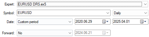
Fig 8: Be sure you have selected dates that are beyond the model's training set
We generally want to stress test our model, so select "Random delay" and "Every tick based on real ticks" to test our strategy under realistic and challenging market conditions.
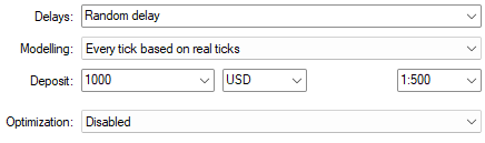
Fig 9: Using "Every tick based on real ticks" is the most realistic modelling choice we can select to stress test our DRS architecture
Below we can find a detailed summary of the performance of our new DRS strategy. It is interesting to realize that we managed to substitute RMSE for DRS and still produced a profitable strategy, even though this was our first attempt to substitute RMSE from our model building process in a formal manner.
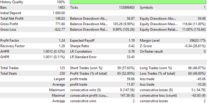
Fig 10: Detailed results of our strategy's performance on data it had not seen before
When we look at the equity curve produced by our strategy, we can start to see the problems caused by our DRS model failing to anticipate market volatility as we discussed before. This causes our strategy to oscillate between profitable periods and unprofitable periods. However, our strategy is demonstrating an ability to recover and stay on track, which is what we desire.

Fig 11: The equity curve produced by our new trading strategy
Conclusion
After reading this article, readers who were not aware of the limitations of these metrics leave stronger than they were when they started this article. Knowing the limitations of your tools is just as important as knowing their strengths. The optimization methods we use to build AI can get "stuck" when trying to solve particularly challenging problems. And when practitioners use these tools to model asset returns, they should be fully aware that their models may demonstrate a tendency to get stuck, at the average return of the market.
The reader has also gained actionable insights and now understands the benefits of filtering markets by how well they can outperform a model predicting the average return in that market because this implies that the market has inefficiencies the practitioner should take advantage of.
By filtering markets based on how well the practitioner can outperform the mean, then reader has learned to desist blindly interpreting RMSE as a standalone metric, and rather read RMSE relative to TSS at all times. The reader has benefited in a practical understanding of the limitations these metrics impose on their everyday work, a feature that is not common in most literature covering this subject, or in the research papers linked here.
And lastly, if the reader were intending on deploying a machine learning model to trade their private capital soon, but he was not aware of these limitations, then I'd caution the reader to first repeat the exercise I demonstrated in this article, to be confident that they were not about to silently shoot themselves in the foot. RMSE allows our models to cheat on our tests, but I have confidence that readers who have read this far, will not be easily fooled by the limitations of AI.
| File Name | File Description |
|---|---|
| DRS Models.mq5 | The MQL5 script we built to fetch the detailed market data we needed to build our DRS model. |
| Dynamic_Regime_Switching_Models_(DRS_Modelling).ipynb | The Jupyter notebook we wrote to design our DRS model. |
| EURUSD DRS.mq5 | Our EURUSD expert advisor that employed our DRS model. |
| EURUSD RF D1 T DRS.onnx | The trend following DRS model always assumes the market is trending. |
| EURUSD RF D1 M DRS.onnx | The mean reverting DRS model always assumes the market is in a mean reverting state. |
Warning: All rights to these materials are reserved by MetaQuotes Ltd. Copying or reprinting of these materials in whole or in part is prohibited.
This article was written by a user of the site and reflects their personal views. MetaQuotes Ltd is not responsible for the accuracy of the information presented, nor for any consequences resulting from the use of the solutions, strategies or recommendations described.

- Free trading apps
- Over 8,000 signals for copying
- Economic news for exploring financial markets
You agree to website policy and terms of use
"However, our strategy demonstrates the ability to recover and stay on track, which is exactly what we strive for."
I always thought that what one should strive for is for a strategy to generate profits :)
"However, our strategy demonstrates the ability to recover and stay on track, which is exactly what we are aiming for."
I've always thought that one should strive for a strategy to bring profits :)
Yes indeed, but unfortunately we still have no standardised machine learning metrics that are aware of the difference between profit and loss.
Thanks for the article, @Gamuchirai Zororo Ndawana
I agree with @Maxim Dmitrievsky that the ultimate goal is profitability. The idea of "recover and stay on track" makes sense as robustness and drawdown control, but it does not replace profit.
Practical suggestion: walk-forward testing, costs and slippage, asymmetric or quantile loss or utility-based objectives, and penalizing turnover to avoid mean hugging. (Pragmatic take: align the loss with how you make money.)
Quoted: Yes indeed, but unfortunately we still have no standardised machine learning metrics that are aware of the difference between profit and loss.
Answer: Profit and loss columns will only exist if your back tested product or the flat market is as good as the forward market you are using against the subsequence portfolio or basket of index that will follow this line of order.
There are some index and newly foundered ETF`s coming out, or that are produced on an increasing basis, as for this intended usage, and will produce these results, profit margins such as the dowjones 30 index as well many other index's which have been created for this intended use. Peter Matty
Thanks for the article, @Gamuchirai Zororo Ndawana
I agree with @Maxim Dmitrievsky that the ultimate goal is profitability. The idea of recovering and staying on track makes sense for robustness and controlling drawdown, but it's no substitute for profit.
Sometimes I wonder if the translation tools we rely on may fail to capture the original message. Your response offers a lot more talking points than what I understood from @Maxim Dmitrievsky original message.
Thank you for pointing out those oversights in the look ahead bias (features with i + HORIZON), those are the worst bugs I hate, they neccisate an entire re-test. But this time more thoughtfully.
You've also provided valuable feedback with the validation measures used to validate models in practice, Sharpe Ratio's must be akin to a universal Gold Standard. I need to learn more about Calmar and Sortino to develop an opinion on those, thank you for that.
I agree with you that the two terms are antisymmetric by design, and the test is that the models should remain antisymmetric, any deviation from this expectation, is failing the test. If one or both models have unacceptable bias then their predictions will not remain antisymmetric as we expect.
However, the notion of profit is only a simple illustration I gave to highlight the problem. None of the metrics we have today inform us when mean hugging is happening. None of the literature on statistical learning tells us why mean hugging is happening. Unfortunately it's happening due to the best practices we follow, and this is just one of many ways I wish to get more conversations started on the dangers of best practices.
This article was more of a cry for help, for us to come together and design new protocols from the ground up. New standards. New objectives that our optimisers work on directly, that are tailored for our interests.