Overcoming The Limitation of Machine Learning (Part 9): Correlation-Based Feature Learning in Self-Supervised Finance

There are many obstacles that make it materially challenging for any member of our community to safely deploy machine-learning-driven trading applications. In this series of articles, we aim to bring to the reader’s attention sources of error that are harder to see and not addressed in standard machine-learning literature. Among these, one of the most consequential is the silent failure that occurs when a model’s underlying assumptions are violated.

All statistical models make certain assumptions about the data you have on hand and the process that generated that data. The fewer assumptions a model makes, the more flexible—or “powerful”—it becomes, as models with fewer assumptions can learn many complex relationships. At this point, some readers may begin thinking, “If models become more powerful by making fewer assumptions, then why not design a model that makes no assumptions whatsoever?” Sadly, it is impossible to build a statistical model that makes no assumptions at all about the data you have. One of the most important assumptions necessary to build a machine learning model is the assumption that there is a relationship between the inputs you have, and the target you are interested in. 

These assumptions form the foundation of our ability, or lack of ability, to profitably forecast any financial market we choose. When these assumptions are violated, nothing happens visibly. There is no warning. This silent point of failure is something current statistical models simply run into at some stage, often without detection.

Academic texts often provide statistical tests to determine whether a model’s assumptions hold. It is important to know how well your model’s assumptions align with the nature of the problem you have, because this tells us whether the model we selected is in sound health for the task we want to delegate to it. However, these standard statistical tests introduce an additional set of material challenges, to an already difficult objective. In brief, standard academic solutions are not only difficult to execute and interpret carefully, but they are also vulnerable to producing false results—meaning they may pass a model that is not sound. This leaves practitioners exposed to unmitigated risks.

Therefore, this article proposes a more practical solution to ensure that your model’s assumptions about the real world are not being violated. We focus on one assumption shared by all statistical models—from simple linear models to modern deep neural networks. All of them assume that the target you have selected is a function of the observations you have on hand. We show that higher levels of performance can be reached by treating the given set of observations as raw material from which we generate new candidate targets that may be easier to learn. This paradigm is also known as self-supervised learning.

These new targets generated from the input data are, by their very definition, guaranteed to be functions of the objective. Doing so may seem unnecessary, but in fact it fortifies one of our statistical models’ greatest blind spots, helping us build more robust and reliable numerically driven trading applications. Let us get started.

Fetching Our Data From The MetaTrader 5 Terminal

In this discussion, we aim to use our inputs, Open, High, Low, and Close (OHLC) price feeds, as the raw ingredients for new supervisory signals our statistical model can learn. Therefore, for reproducibility, it is best that we perform all manipulations to the data in MQL5. In machine learning, the objective, future price is assumed to be a function of the observations, OHLC. This violates standard portfolio theory, because we know future returns are a function of investor expectations, not historical prices. With this motivation, let us calculate new imaginary points that lie in between the observed price levels. To do so in MQL5, we apply simple arithmetic to compute the imaginary midpoint that sits between each pair of OHLC feeds.

//+------------------------------------------------------------------+
//|                                            Fetch Data Mid Points |
//|                                      Copyright 2020, CompanyName |
//|                                       http://www.companyname.net |
//+------------------------------------------------------------------+
#property copyright "Copyright 2024, MetaQuotes Ltd."
#property link      "https://www.mql5.com"
#property version   "1.00"
#property script_show_inputs

//--- File name
string file_name = Symbol() + " Mid Points.csv";

//--- Amount of data requested
input int size = 3000;

//+------------------------------------------------------------------+
//| Our script execution                                             |
//+------------------------------------------------------------------+
void OnStart()
  {
   
//---Write to file
   int file_handle=FileOpen(file_name,FILE_WRITE|FILE_ANSI|FILE_CSV,",");

   for(int i=size;i>=1;i--)
     {
      if(i == size)
        {
         FileWrite(file_handle,
                  //--- Time
                  "Time",
                   //--- OHLC
                   "Open",
                   "High",
                   "Low",
                   "Close",
                   //--- OHLC Mid Points
                   "O-H M",
                   "O-L M",
                   "O-C M",
                   "H-L M",
                   "H-C M",
                   "L-C M"
                  );
        }

      else
        {
         FileWrite(file_handle,
                   iTime(_Symbol,PERIOD_CURRENT,i),
                   //--- OHLC
                   iOpen(_Symbol,PERIOD_CURRENT,i),
                   iHigh(_Symbol,PERIOD_CURRENT,i),
                   iLow(_Symbol,PERIOD_CURRENT,i),
                   iClose(_Symbol,PERIOD_CURRENT,i),
                   //--- OHLC Mid Points
                    (iOpen(_Symbol,PERIOD_CURRENT,i) +  iHigh(_Symbol,PERIOD_CURRENT,i))/2,
                    (iOpen(_Symbol,PERIOD_CURRENT,i) +  iLow(_Symbol,PERIOD_CURRENT,i))/2,
                    (iOpen(_Symbol,PERIOD_CURRENT,i) +  iClose(_Symbol,PERIOD_CURRENT,i))/2,
                    (iHigh(_Symbol,PERIOD_CURRENT,i) +  iLow(_Symbol,PERIOD_CURRENT,i))/2,
                    (iHigh(_Symbol,PERIOD_CURRENT,i) +  iClose(_Symbol,PERIOD_CURRENT,i))/2,
                    (iLow(_Symbol,PERIOD_CURRENT,i) +  iClose(_Symbol,PERIOD_CURRENT,i))/2
                   );
        }
     }
//--- Close the file
   FileClose(file_handle);
  }
//+------------------------------------------------------------------+

Analyzing Our Market Data in Python

Let us start by first importing our standard Python libraries.

#Load our libraries
import pandas as pd
import numpy as np
import seaborn as sns
import matplotlib.pyplot as plt

Next, read in the CSV file we generated using our MQL5 script.

#Read in the data
data = pd.read_csv('./EURUSD Mid Points.csv')
data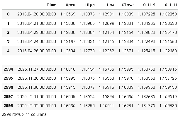

Figure 1: Visualizing our market data as we calculated in our MQL5 script

We calculated midpoints in our MQL5 script using our understanding of arithmetic. However, we should perform some tests for correctness to ensure we implemented what we were envisioning. As we can see in Figure 2 below, we have plotted the historical EURUSD high and low exchange rates as we received them from our broker. Additionally, we can observe the dashed imaginary midpoint we calculated in MQL5 sits in between the high and the low, as we expected.

#Examine correctness
plt.plot(data.loc[0:10,'High'],color='red')
plt.plot(data.loc[0:10,'H-L M'],color='black',linestyle=':')
plt.plot(data.loc[0:10,'Low'],color='blue')
plt.grid()
plt.legend(['High','H-L Mid','Low'])
plt.ylabel('EURUSD Exchange Rate')
plt.xlabel('Hisotircal Time Stamp')
plt.title('The High-Low Mid Point of EURUSD Exchange Rates')

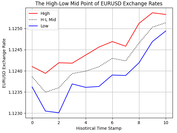
Figure 2: Visualizing the Midpoint between the EURUSD High & Low Price

The midpoint between the open and close prices was also calculated correctly, as we can observe in the illustration that follows.

#Examine correctness
plt.plot(data.loc[70:90,'Open'],color='red')
plt.plot(data.loc[70:90,'O-C M'],color='black',linestyle=':')
plt.plot(data.loc[70:90,'Close'],color='blue')
plt.grid()
plt.legend(['Open','O-C Mid','Close'])
plt.ylabel('EURUSD Exchange Rate')
plt.xlabel('Hisotircal Time Stamp')
plt.title('The Open-Close Mid Point of EURUSD Exchange Rates')

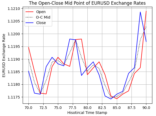
Figure 3: Visualizing the Midpoint between the open and close price.

Now, let us define how far into the future we wish to forecast.

#Forecast horizon
HORIZON = 2

Normally, in standard academic literature on statistical learning, it is at this point where the reader is expected to separate their inputs and their target. However, this is the hallmark distinction of the solution this article aims to leave the reader with. Instead of working with a fixed target in mind, we will generate as many targets as we can from the observations we have.

#Candidate targets
candidate_y = data.iloc[:,4:11].columns
candidate_x = data.iloc[:,1:5].columns

For this exercise, we have kept the classical target of future price, and additionally we have other surrogate targets that we believe may be easier to learn than the classical target.

candidate_y

Index(['Close', 'O-H M', 'O-L M', 'O-C M', 'H-L M', 'H-C M', 'L-C M'], dtype='object')

Create columns in the original dataset to store the future value of each candidate target.

data['Label 1'] = 0
data['Label 2'] = 0
data['Label 3'] = 0
data['Label 4'] = 0
data['Label 5'] = 0
data['Label 6'] = 0
data['Label 7'] = 0

Finally, create additional columns to stand as binary targets for each target we wish to assess.

data['Target 1'] = 0
data['Target 2'] = 0
data['Target 3'] = 0
data['Target 4'] = 0
data['Target 5'] = 0
data['Target 6'] = 0
data['Target 7'] = 0

We need to now label our dataset and then fill in the target value. This simple loop will iteratively fill in the columns of 0’s we defined previously with the future value of the target and its respective binary representation.

#Label the dataset
for i in np.arange(7):
  #Add labels to the data
  label = 'Label ' + str(i+1)
  data[label] = data[candidate_y[i]].shift(-HORIZON)
  #Define the labels as binary targets
  target = 'Target ' + str(i+1)
  data[target] = 0
  #Add the target
  data.loc[data[label] > data[candidate_y[i]],target] = 1

#Drop the last missing forecast horizon period
data = data.iloc[:-HORIZON,:]
data

Now, let us load the statistical learning libraries we need to determine which target is easier for our model to learn, given the observations on hand.

from sklearn.model_selection import TimeSeriesSplit,cross_val_score
from sklearn.discriminant_analysis import LinearDiscriminantAnalysis

To keep our comparisons rigorous, we will use the same model with each target.

def get_model():
  return(LinearDiscriminantAnalysis())

Now define our time series cross-validation object. This ensures we will not perform random shuffling when cross-validating our model.

tscv = TimeSeriesSplit(n_splits=5,gap=HORIZON)

Prepare an array to keep track of our accuracy on each target.

scores = []

Cross-validate the performance of the same model, given the same inputs, but only change the target the model is trying to learn from the observations it has.

#Classical Target
scores.append(np.mean(cross_val_score(get_model(),data.loc[:,candidate_x],data.iloc[:,-7],cv=tscv,scoring='accuracy')))

#Modern Targets
scores.append(np.mean(cross_val_score(get_model(),data.loc[:,candidate_x],data.iloc[:,-6],cv=tscv,scoring='accuracy')))
scores.append(np.mean(cross_val_score(get_model(),data.loc[:,candidate_x],data.iloc[:,-5],cv=tscv,scoring='accuracy')))
scores.append(np.mean(cross_val_score(get_model(),data.loc[:,candidate_x],data.iloc[:,-4],cv=tscv,scoring='accuracy')))
scores.append(np.mean(cross_val_score(get_model(),data.loc[:,candidate_x],data.iloc[:,-3],cv=tscv,scoring='accuracy')))
scores.append(np.mean(cross_val_score(get_model(),data.loc[:,candidate_x],data.iloc[:,-2],cv=tscv,scoring='accuracy')))
scores.append(np.mean(cross_val_score(get_model(),data.loc[:,candidate_x],data.iloc[:,-1],cv=tscv,scoring='accuracy')))

Now the reader can clearly see the practical value of our proposed solution. By designing your own targets from the observations you started with, you can attain new error levels you would never attain if you bound yourself to the classical fixed target of future price.

scores

[np.float64(0.503006012024048),

np.float64(0.7082164328657314),

np.float64(0.6941883767535071),

np.float64(0.6328657314629258),

np.float64(0.6501002004008015),

np.float64(0.5739478957915832),

np.float64(0.5739478957915831)]

When we visualize the results of our proposed solution, the improvements we have made become self-evident. Our model found it easier to learn every other target we built from the observations than it did trying to learn price itself. It appears the benefits are well worth the additional effort it costs to acquire them.

sns.barplot(scores,color='black')
plt.xticks([0,1,2,3,4,5,6],candidate_y)
plt.axhline(scores[0],linestyle=':',color='red')
plt.ylabel('Accuracy out of 100%')
plt.xlabel('Selected Target')
plt.title('EURUSD Forecasting Accuracy is a Function of The Target')

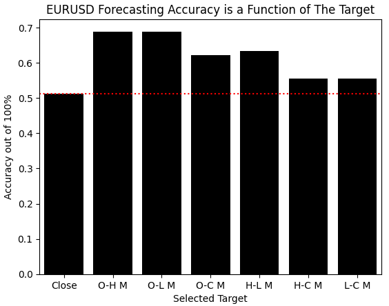
Figure 4: The changes realized by changing our target are remarkable and warrant further exploration

As numerically driven algorithmic traders, we can quickly learn a lot about our dataset from carefully interpreting meaningful numbers taken from our dataset. In this case, we need to be cautious of reward hacking. Therefore, we must ascertain the highest score any model could’ve obtained by always forecasting the most common label for each target.

Since each target is either 1 or 0, calculating the mean of each target actually informs us which target value is the most common and its ratio of dominance. If the two target values are appearing equally, then the average value of that target should be 0.5. Deviations beneath 0.5 imply that more 0s were present, and the converse implies more 1s were present. The mean can only be 1 if all target values were 1, and likewise all entries must be 0 to obtain a mean of 0.

Therefore, we can see that our candidate targets are well behaved, and none of them deviated too far from 0.5 to reasonably explain the improvements over the classical model.

data.iloc[:,-7:].mean()

Target	Average
Target 1	0.502836
Target 2	0.507174
Target 3	0.487154
Target 4	0.494161
Target 5	0.500167
Target 6	0.474808
Target 7	0.522856

Now that we have identified targets easier to predict than the original price levels, let us now learn how our new target is related to the classical target. This is a critical step. We start by importing a simple linear model

from sklearn.linear_model import LinearRegression

Statistical tools can be used for inference or for insight. We normally use our tools for inference, or simply forecasting. Today, we will turn our attention to using these models for insight, not for predictive modeling.

explanation = LinearRegression()

Fitting a linear model on two targets may appear unfounded at first. However, it is perfectly sound practice.

explanation.fit(data[['Label 1']],data['Label 2'])

The coefficients learned by our linear model immediately tell us if our two targets move together or if they move in opposite directions. Our linear model estimated coefficients almost equal to 1, meaning that the new target we have generated follows the classical target almost perfectly. And therefore, forecasting the new target is just as good as forecasting the classical target, with the advantage that the new target we formulated is less expensive to learn.

explanation.coef_

array([0.99533718])

Alternatively, the reader could also just have calculated the correlation matrix of the candidate targets we generated to arrive at the same realization.

data.iloc[:,-14:-7].corr()

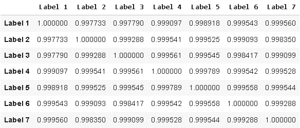
Figure 5: Visualizing the correlation between the candidate targets we have designed and the classical target

Finally, we can also prove this to ourselves visually by performing a plot of the classical target we have against the new target we wish to model. Doing so reveals to us what we confirmed by the insights we obtained from our linear model and the correlation matrix: our two targets follow each other with clear and definite affinity.

plt.plot(data.iloc[0:200,-14],color='black')
plt.plot(data.iloc[0:200,-13],linestyle=':',color='red')
plt.grid()
plt.ylabel('EURUSD Exchange Rate')
plt.xlabel('Historical Time')
plt.title('Visualizing Our Classical & Candidate Target')
plt.legend(['Classical Target','Candidate Target'])

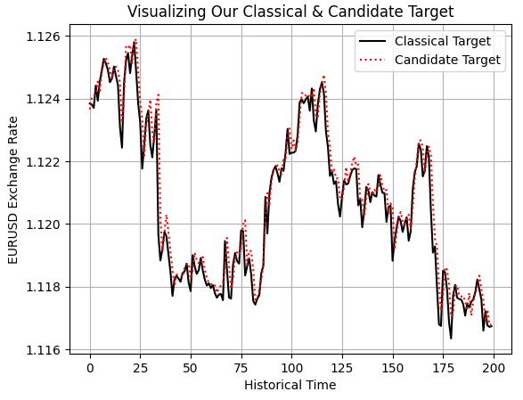
Figure 6: Visualizing the relationship between our engineered candidate target and the classical target

Now that we have identified which target we are learning best, we will now use all the input data we have generated thus far to help us model the target we are excelling on.

X = ['Open','High','Low','Close','O-H M','O-C M', 'H-L M', 'H-C M', 'L-C M']
y = ['Target 2']

To my surprise, our performance levels did not change at all, despite the additional inputs we supplied to our model.

np.mean(cross_val_score(get_model(),data.loc[:,X],data.iloc[:,-6],cv=tscv,scoring='accuracy'))

np.float64(0.7082164328657314)

Recall the score we obtained using ordinary OHLC price data.

scores[1]

np.float64(0.7082164328657314)

Before we can conclude that we have realized the best statistical model possible, we must be confident that we cannot improve our performance by creating a more detailed description of the market’s behavior for our model. Therefore, we will calculate growth in individual price feeds, and additionally, we will also calculate growth across different price feeds. All these features will be aggregated with the original batch of features we started with, giving us a high-dimensional and detailed perspective on the EURUSD exchange rates.

#Feature Engineering
initial_features = data.loc[:,X]

#Growth in individual Price Levels
new_features = initial_features

new_features['Delta Open']  = data['Open'].shift(HORIZON)  - data['Open']
new_features['Delta High']  = data['High'].shift(HORIZON)  - data['High']
new_features['Delta Low']   = data['Low'].shift(HORIZON)   - data['Low']
new_features['Delta Close'] = data['Close'].shift(HORIZON) - data['Close']

#Growth across all Price levels
new_features['Growth O-H'] = data['Open'].shift(HORIZON) - data['High'].shift(HORIZON)
new_features['Growth O-L'] = data['Open'].shift(HORIZON) - data['Low'].shift(HORIZON)
new_features['Growth O-C'] = data['Open'].shift(HORIZON) - data['Close'].shift(HORIZON)
new_features['Growth H-L'] = data['High'].shift(HORIZON) - data['Low'].shift(HORIZON)
new_features['Growth H-C'] = data['High'].shift(HORIZON) - data['Close'].shift(HORIZON)
new_features['Growth L-C'] = data['Low'].shift(HORIZON)  - data['Close'].shift(HORIZON)

new_features = new_features.iloc[HORIZON:,:]
new_features.reset_index(drop=True,inplace=True)

data = data.loc[HORIZON:,:]
data.reset_index(inplace=True,drop=True)

new_features

Our intuition may have led us to believe that such an approach is guaranteed to bring about improvements; however, in this series of articles we aim to give voice to the numbers and let the data speak for itself. It appears that all our effort in cultivating those new features was in vain because we are still failing to outperform an identical model that was constrained to observe far less data.

np.mean(cross_val_score(get_model(),new_features,data.iloc[:,-6],cv=tscv,scoring='accuracy'))

np.float64(0.688118007375461)

For readers who need a refresher, this is the score we are attempting to beat. Feature engineering is a necessary step to ensure that we are using the best model possible for the data we have. It is not guaranteed to improve your results. As all returning readers should be familiar with by now, in optimization there are no guarantees.

scores[1]

np.float64(0.6889680605037813)

At this stage, we have exhausted feature engineering based on direct transformations of the raw price feeds. Since these additional descriptive features failed to yield improvements, our next question becomes whether the information contained in the dataset is better expressed in a different coordinate system altogether.

Some relationships may be difficult to learn in high-dimensional settings, and therefore could it be possible that our model could learn these relationships better in a more meaningful low dimensional representation of the original dataset? This question is answered by a family of statistical algorithms known as manifold learning techniques. In this discussion, we will employ Independent Component Analysis (ICA) as our manifold learning algorithm choice.

ICA is a powerful extension of the popular Principal Component Analysis algorithm (PCA). Among many differences, PCA can be computed quickly because it relies on closed form solutions expressed in linear algebra. However, ICA is better conceived of as an optimization problem that does not have a closed solution, but rather it must be attempted iteratively.

ICA was popularized by the signal processing community, where it was found to be capable of isolating and separating signals that may have interfered with each other. ICA is effectively capable of reducing any given matrix of data into maximally independent and non-Gaussian vectors believed to be the original sources of the signal that generated the observations. Readers interested in gaining a deeper appreciation of ICA can find a well written research article on the subject, linked, here.

#Manifold Learning
from sklearn.decomposition import FastICA
from sklearn.model_selection import RandomizedSearchCV

Typically, high-dimensional datasets can be challenging to learn from. Manifold learning techniques such as FastICA are motivated by the belief that although the data is recorded in high-dimensional space, most of the dimensions are only ambient space, and the real process we are interested in may be dominated by only a few important dimensions. Therefore, we will iteratively allow our FastICA algorithm to represent our original market data of 20 columns using 1 until 18 columns, and we record our performance each time.

#Keep track of our performance
manifold = []

#Search for a manifold where the objective is easier to learn
res = []

for i in np.arange(new_features.shape[1]-2):
  enc = FastICA(n_components=i+1)
  new_manifold = pd.DataFrame(enc.fit_transform(new_features))
  res.append(np.mean(cross_val_score(get_model(),new_manifold,data.iloc[:,-6],cv=tscv,scoring='accuracy')))

#Remember the score we are trying to outperform
res.append(scores[1])

As we can observe, our best results were obtained on the last bar plot, representing that a model only using OHLC data would’ve still outperformed us, even after applying FastICA. Therefore, at this point we can be confident that we have an optimal model just by simply using the OHLC market data, and we can now export our model to ONNX format with confidence.

sns.barplot(res,color='black')
plt.axhline(np.max(res),color='red',linestyle=':')
plt.scatter(np.argmax(res),np.max(res),color='red')

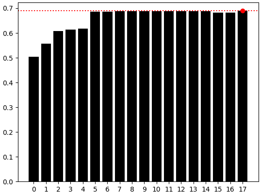
Figure 7: The simple model using 4 columns (OHLC) was still our best performing model

Exporting To ONNX

We are now ready to export our statistical model to the Open Neural Network Exchange format, also known as ONNX. ONNX allows us to efficiently and operatively share our machine-learning model and express our model in a platform-agnostic manner. Therefore, we load the necessary libraries. 

import onnx
from skl2onnx.common.data_types import FloatTensorType
from skl2onnx import convert_sklearn

Define the input shape of the model. The model takes four primary price feeds, and these input types are of type float, which we specify using the float template type. 

initial_types = [('float_input',FloatTensorType([1,4]))]

We also specify the output shape of the model: the model has one output—the target.

final_types = [('float_output',FloatTensorType([1,1]))]

Afterward, we need to enforce a separation of inputs. We do not want to train our model on the same time period that we intend to back-test in MetaTrader 5. Therefore, we drop the last five years from our dataset and keep the remainder as the training set. 

train = data.iloc[:(-365*5),:]
test = data.iloc[(-365*5):,:]

Random forests are powerful and flexible statistical models that can learn nonlinear effects in the data. So we load the random forest model in this discussion, although the reader is free to load any model of choice. 

In this example, we use the ATR to set our stop losses according to market volatility. Everything else will be handled first by our model.

from sklearn.ensemble import RandomForestRegressor

Then we fit the model on our training data.

model = RandomForestRegressor()

model.fit(data.loc[:,['Open','High','Low','Close']],data.loc[:,'Label 2'])

From there, we prepare to convert the model into its ONNX prototype. This prototype is an intermediary file before we save our ONNX model to drive.

onnx_proto = convert_sklearn(model,initial_types=initial_types,final_types=final_types,target_opset=12)

Now we can save the ONNX file.

onnx.save(onnx_proto,'EURUSD MidPoint RFR.onnx')

Testing Our Assumptions

We are now ready to begin building the application. We start by loading the ONNX file we just wrote to disk.

//+------------------------------------------------------------------+
//|                                              EURUSD MidPoint.mq5 |
//|                                  Copyright 2025, MetaQuotes Ltd. |
//|                                             https://www.mql5.com |
//+------------------------------------------------------------------+
#resource "\\Files\\EURUSD MidPoint RFR.onnx" as const uchar onnx_proto[];

And then we define the technical indicators that we will need.

//+------------------------------------------------------------------+
//| Technical Indicators                                             |
//+------------------------------------------------------------------+
int      atr_handler;
double   atr_reading[];

We also need a few global variables to track the current bid and ask prices, as well as a few important functions for our model, such as the handler and the model’s inputs and outputs.

//+------------------------------------------------------------------+
//| Global variables                                                 |
//+------------------------------------------------------------------+
double  ask,bid;
vectorf model_inputs,model_outputs;
long    model;

Then we load the trade library to help us manage our position entries and exits. 

//+------------------------------------------------------------------+
//| Libraries                                                        |
//+------------------------------------------------------------------+
#include <Trade\Trade.mqh>
CTrade Trade;

When our application loads for the first time, we then load the appropriate technical indicators and begin initializing our model from the ONNX export that we created earlier. We set the input and output shapes, and finally we check if the model is valid before handing control back to the calling instance.

//+------------------------------------------------------------------+
//| Expert initialization function                                   |
//+------------------------------------------------------------------+
int OnInit()
  {
//--- Setup our indicators
   atr_handler     = iATR("EURUSD",PERIOD_D1,14);

//--- Setup the ONNX model
   model = OnnxCreateFromBuffer(onnx_proto,ONNX_DATA_TYPE_FLOAT);

//--- Define the model parameter shape
   ulong input_shape[] = {1,4};
   ulong output_shape[] = {1,
    1 };

   OnnxSetInputShape(model,0,input_shape);
   OnnxSetOutputShape(model,0,output_shape);

   model_inputs = vectorf::Zeros(4);
   model_outputs = vectorf::Zeros(
    1 );

   if(model != INVALID_HANDLE)
     {
      return(INIT_SUCCEEDED);
     }

//---
   return(INIT_FAILED);
  } 

When our application is no longer in use, we release the resources that were dedicated to the technical indicator and the ONNX model.

//+------------------------------------------------------------------+
//| Expert deinitialization function                                 |
//+------------------------------------------------------------------+
void OnDeinit(const int reason)
  {
//--- Free up memory we are no longer using when the application is off
   IndicatorRelease(atr_handler);
   OnnxRelease(model);
  }

Whenever new price levels are received, we update our current record of the time, and if a new daily candle has formed, we fetch fresh copies of the current price levels and then recalculate our imaginary midpoint according to the current prices. We then pass the ONNX model its four inputs and obtain a prediction. If our model expects the midpoint in the future to be greater than where it is now, we enter long positions; otherwise, we enter short positions.

//+------------------------------------------------------------------+
//| Expert tick function                                             |
//+------------------------------------------------------------------+
void OnTick()
  {
//--- When price levels change

   datetime current_time = iTime("EURUSD",PERIOD_D1,0);
   static datetime  time_stamp;

//--- Update the time
   if(current_time != time_stamp)
     {
      time_stamp = current_time;

      //--- Fetch indicator current readings
      CopyBuffer(atr_handler,0,0,1,atr_reading);

      double open = iOpen("EURUSD",PERIOD_D1,0);
      double close = iClose("EURUSD",PERIOD_D1,0);
      double high = iHigh("EURUSD",PERIOD_D1,0);
      double low = iLow("EURUSD",PERIOD_D1,0);
            double o_h_mid = ((open + high)/2);

      model_inputs[0] = (float) open;
      model_inputs[1] = (float) high;
      model_inputs[2] = (float) low;
      model_inputs[3] = (float) close;

      ask = SymbolInfoDouble("EURUSD",SYMBOL_ASK);
      bid = SymbolInfoDouble("EURUSD",SYMBOL_BID);

      //--- If we have no open positions
      if(PositionsTotal() == 0)
        {

         if(!(OnnxRun(model,ONNX_DATA_TYPE_FLOAT,model_inputs,model_outputs)))
           {
            Comment("Failed to obtain a forecast from our model: ",GetLastError());
           }

         else
           {
            Comment("Forecast: ",model_outputs);

            //--- Trading rules
            if((model_outputs[1] > o_h_mid))
              {
               //--- Buy signal
               Trade.Buy(0.01,"EURUSD",ask,ask-(atr_reading[0] * 2),ask+(atr_reading[0] * 2),"");
              }

            else
               if((model_outputs[1] < o_h_mid))
                 {
                  //--- Sell signal
                  Trade.Sell(0.01,"EURUSD",bid,bid+(atr_reading[0] * 2),bid-(atr_reading[0] * 2),"");
                 }
           }
        }
     }
  }
//+------------------------------------------------------------------+

We are now ready to begin the five-year backtest of our model from February 2020 until the time of writing in 2025.

Figure 8: Selecting the backtest days for our 5 year test of our new assumptions

We set random delay settings to obtain a realistic emulation of network delays and other latencies experienced in live trading. 

Figure 9: Ensure you select random delay settings for a robust emulation of real market conditions

When the test completes, we can observe the equity curve produced by the approach suggested in this article. As you can see, even though the model is as simple as possible, it produces a dominant uptrend in the equity curve over five years of trading. It uses all signals, which is astounding for a model this simple—showing that there is merit in self-supervised learning.

Figure 10: The new equity curve produced by our new assumptions

Additionally, when we examine the detailed statistics of the model’s performance, we see a healthy profit factor and a healthy expected payoff. Producing values greater than one indicates that the model appreciated in profit over five years. However, it is disappointing to see that the model’s trades are biased once again toward long trades: the model entered almost three times more long positions than short positions over five years. This indicates that there are still weaknesses and blind spots that we have not yet covered. Although the random forest model should be capable of learning strong nonlinear relationships, it is interesting to note that bias still appears in the model.

Figure 11: The detailed statistics of the performance of our new statistical strategy

Conclusion

In conclusion, this article has demonstrated how higher-order statistical signals can be realized in a self-supervised fashion and applied in an algorithmic trading setup. By relying only on the data received from our broker, we can generate new signals that our statistical models can learn more reliably. Even a simple model built with a self-supervised paradigm appears robust enough to be left unsupervised for five years and still perform soundly. Additionally, the article has shown the reader how to search for more inputs that they can use to improve accuracy—and not to assume that more data automatically improves results, but instead to empirically test whether more data truly helps. As we have seen in this article, even the bare necessities can be used as powerful trading signals.

Lastly, as we have discussed extensively in the opening article of this series of articles, the performance metrics we use to critique statistical models are not necessarily interoperable with our objectives as a community of algorithmic traders. Therefore, the reader should note that the model's statistical accuracy of 68%, only materialized to 52% profitability in our discussion. 

File Name	File Description
Self Supervised Learning: Generating Targets From OHLC Data.ipynb	The Jupyter Notebook we used to perform our statistical analysis on our historical EURUSD market data.
EURUSD MidPoint.mq5	The trading application we built to take its trading signals based on self-supervised signals it learned.
Fetch Data Mid Points.mq5	The MQL5 script we used to fetch and manipulate our historical EURUSD market data.