
Overcoming The Limitation of Machine Learning (Part 7): Automatic Strategy Selection

When most traders begin their journey, they’re advised to choose strategies that match their risk profile. While this is reasonable, this article petitions to the reader that trading strategies should be first discovered based on expected performance levels rather than idealized preferences. Identifying profitable strategies is a universal challenge for algorithmic traders, regardless of experience. The difficulty is compounded by the constant flow of new strategies, indicators, and expert advisors emerging from our rapidly growing global community of algorithmic traders.
We live in an age of unprecedented interconnectivity—an informational revolution. But what happens when new ideas appear and spread faster than any trader can evaluate them? Given countless possible strategies, how can we automatically identify a shortlist we believe is worth testing? Can we discover potentially profitable configurations of strategies, without brute-forcing every possible combination?
This article proposes a framework to address these questions through two complementary approaches:
- White Box Solution: Use matrix factorization—specifically singular value decomposition (SVD)—on expected returns to identify strategy combinations positively influenced by current market conditions.
- Black Box Solution: Employ deep neural networks to dynamically select strategies based on observed market behavior.
Our solution relies on our ability to estimate the returns that would've been generated by following the trading strategies on hand. We then leverage our understanding of numerical computing to learn the expected revenue streams from our strategies. There is valuable insight to be gained from approximating the returns generated by any given strategy.
Fetching The Data We Need
To get started, we will first write out an MQL5 script to fetch the important market data we need. We will fetch ordinary market data and also fetch data related to the indicator inputs to ensure that our ONNX models will be trained on the same indicator calculations they will observe in production.
//+------------------------------------------------------------------+
//|                                                      ProjectName |
//|                                      Copyright 2020, CompanyName |
//|                                       http://www.companyname.net |
//+------------------------------------------------------------------+
#property copyright "Copyright 2024, MetaQuotes Ltd."
#property link      "https://www.mql5.com"
#property version   "1.00"
#property script_show_inputs

//--- Define our moving average indicator
#define MA_PERIOD     5                   //--- Moving Average Period
#define MA_TYPE       MODE_SMA            //--- Type of moving average we have

#define RSI_PERIOD    15                  //--- RSI Period

#define STOCH_K       5                    //--- Stochastich K Period
#define STOCH_D       3                    //--- Stochastich D Period
#define STOCH_SLOWING 3                    //--- Stochastic slowing
#define STOCH_MODE    MODE_EMA             //--- Stochastic mode
#define STOCH_PRICE   STO_LOWHIGH          //--- Stochastic price feeds

#define HORIZON        5                   //--- Forecast horizon

//--- Our handlers for our indicators
int ma_handle,ma_o_handle,ma_h_handle,ma_l_handle,rsi_handle,stoch_handle;

//--- Data structures to store the readings from our indicators
double ma_reading[],ma_o_reading[],ma_h_reading[],ma_l_reading[],rsi_reading[],sto_reading_main[],sto_reading_signal[];

//--- File name
string file_name = Symbol() + " Market Data As Series Indicators.csv";

//--- Amount of data requested
input int size = 3000;

//+------------------------------------------------------------------+
//| Our script execution                                             |
//+------------------------------------------------------------------+
void OnStart()
  {
   int fetch = size + (HORIZON * 2);
//---Setup our technical indicators
   ma_handle = iMA(_Symbol,PERIOD_CURRENT,MA_PERIOD,0,MA_TYPE,PRICE_CLOSE);
   ma_o_handle = iMA(_Symbol,PERIOD_CURRENT,MA_PERIOD,0,MA_TYPE,PRICE_OPEN);
   ma_h_handle = iMA(_Symbol,PERIOD_CURRENT,MA_PERIOD,0,MA_TYPE,PRICE_HIGH);
   ma_l_handle = iMA(_Symbol,PERIOD_CURRENT,MA_PERIOD,0,MA_TYPE,PRICE_LOW);
   rsi_handle  = iRSI(_Symbol,PERIOD_CURRENT,RSI_PERIOD,PRICE_CLOSE);
   stoch_handle = iStochastic(_Symbol,PERIOD_CURRENT,STOCH_K,STOCH_D,STOCH_SLOWING,STOCH_MODE,STOCH_PRICE);

//---Set the values as series
   CopyBuffer(ma_handle,0,0,fetch,ma_reading);
   ArraySetAsSeries(ma_reading,true);
   CopyBuffer(ma_o_handle,0,0,fetch,ma_o_reading);
   ArraySetAsSeries(ma_o_reading,true);
   CopyBuffer(ma_h_handle,0,0,fetch,ma_h_reading);
   ArraySetAsSeries(ma_h_reading,true);
   CopyBuffer(ma_l_handle,0,0,fetch,ma_l_reading);
   ArraySetAsSeries(ma_l_reading,true);
   CopyBuffer(rsi_handle,0,0,fetch,rsi_reading);
   ArraySetAsSeries(rsi_reading,true);
   CopyBuffer(stoch_handle,0,0,fetch,sto_reading_main);
   ArraySetAsSeries(sto_reading_main,true);
   CopyBuffer(stoch_handle,0,0,fetch,sto_reading_signal);
   ArraySetAsSeries(sto_reading_signal,true);

//---Write to file
   int file_handle=FileOpen(file_name,FILE_WRITE|FILE_ANSI|FILE_CSV,",");

   for(int i=size;i>=1;i--)
     {
      if(i == size)
        {
         FileWrite(file_handle,
                  //--- Time
                  "Time",
                   //--- OHLC
                   "Open",
                   "High",
                   "Low",
                   "Close",
                   //--- MA OHLC
                   "MA O",
                   "MA H",
                   "MA L",
                   "MA C",
                   //--- RSI
                   "RSI",
                   //--- Stochastic Oscilator
                   "Stoch Main",
                   "Stoch Signal"
                  );
        }

      else
        {
         FileWrite(file_handle,
                   iTime(_Symbol,PERIOD_CURRENT,i),
                   //--- OHLC
                   iOpen(_Symbol,PERIOD_CURRENT,i),
                   iHigh(_Symbol,PERIOD_CURRENT,i),
                   iLow(_Symbol,PERIOD_CURRENT,i),
                   iClose(_Symbol,PERIOD_CURRENT,i),
                   //--- MA OHLC
                   ma_o_reading[i],
                   ma_h_reading[i],
                   ma_l_reading[i],
                   ma_reading[i],
                   //--- RSI
                   rsi_reading[i],
                   //--- Stochastic Oscilator
                   sto_reading_main[i],
                   sto_reading_signal[i]
                  );
        }
     }
//--- Close the file
   FileClose(file_handle);
  }
//+------------------------------------------------------------------+

//+------------------------------------------------------------------+
//| Undefine system constants                                        |
//+------------------------------------------------------------------+
#undef HORIZON
#undef MA_PERIOD
#undef MA_TYPE
//+------------------------------------------------------------------+
Analyzing The Data We Need
Next, we shall import the standard python libraries we will need.
#Import the standard libraries
import pandas as pd
import numpy as np
import matplotlib.pyplot as plt
import seaborn as sns
First, load the dataset we created using our MQL5 script.
data = pd.read_csv("../EURUSD Market Data As Series Indicators.csv")
Next, partition the dataset to exclude any period that overlaps with the intended backtest window. Including overlapping data would undermine the validity of our results.
#Drop the last 3 years of historical data
data = data.iloc[:-(365*3),:]
_ = data.iloc[-(365*3):,:]
Make sure the forecast horizon aligns with the forecasting period defined in the script.
HORIZON = 5Then calculate the realized market return.
data['Return'] = data['Close'].shift(-HORIZON) - data['Close']
data.dropna(inplace=True)
To estimate each strategy’s return, we must first determine the direction it anticipated the market to move. If the strategy predicted bullish price action, assign a return of 1; if bearish, assign -1. Multiply this anticipated return by the actual return to approximate the strategy’s performance. The return will be positive only when the strategy correctly anticipated the market direction.
data['MA OC Strategy'] = 0
data['MA HL Strategy'] = 0
data['RSI Strategy'] = 0
data['Stochastic Strategy'] = 0

#Moving Average Open and Close strategy
data.loc[data['MA O']<data['MA C'],'MA OC Strategy'] = 1
data.loc[data['MA O']>data['MA C'],'MA OC Strategy'] = -1

#Moving average High Low Strategy
data.loc[data['Close']>data['MA H'],'MA HL Strategy'] = 1
data.loc[data['Close']<data['MA L'],'MA HL Strategy'] = -1

#RSI Strategy
data.loc[data['RSI']>50,'RSI Strategy'] = 1
data.loc[data['RSI']<50,'RSI Strategy'] = -1

#Stoch Main Strategy
data.loc[data['Stoch Main']>80,'Stochastic Strategy'] = 1
data.loc[data['Stoch Main']<30,'Stochastic Strategy'] = -1


#Strategy Returns
for i in np.arange(4):
    data.iloc[:,-1*(i+1)]= data.iloc[:,-1*(i+1)] * data['Return']
    data.iloc[:,-1*(i+1)]= data.iloc[:,-1*(i+1)].cumsum()

data['Return'] = data['Return'].cumsum()
We also want to examine how market returns evolve over multiple time steps.
data['MA OC 1'] = data['MA OC Strategy'].shift(-1)
data['MA OC 2'] = data['MA OC Strategy'].shift(-HORIZON)

data['MA HL 1'] = data['MA HL Strategy'].shift(-1)
data['MA HL 2'] = data['MA HL Strategy'].shift(-HORIZON)

data['RSI 1'] = data['RSI Strategy'].shift(-1)
data['RSI 2'] = data['RSI Strategy'].shift(-HORIZON)


data['Stochastic 1'] = data['Stochastic Strategy'].shift(-1)
data['Stochastic 2'] = data['Stochastic Strategy'].shift(-HORIZON)


data.dropna(inplace=True)

data
Now separate the inputs from the targets.
X = data.iloc[:,1:12]
y = data.iloc[:,-8:]
Next, let’s visualize the anticipated strategy returns. As shown in Figure 1, all four strategies appear unprofitable from the outset. However, this information is still valuable.
plt.plot(data.iloc[:,-12:-8])
plt.legend(data.columns[-12:-8])
plt.grid()
plt.title('Estimating The Effectiveness of Different Strategies')
plt.ylabel('Estimated Profit Level')
plt.xlabel('Historical Training Epochs')
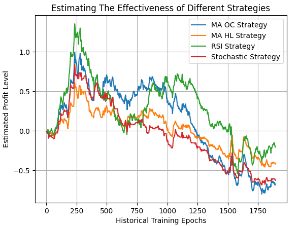
Figure 1: Visualizing the returns of our independent strategies in their present form
We will now perform Singular Value Decomposition (SVD) on the strategy returns.
#Analyze the returns
U,S,VT = np.linalg.svd(data.iloc[:,-12:-8])
SVD reveals the underlying structure in the data, and for this discussion, we’re particularly interested in the number of unique modes of variation the strategies exhibit. Each mode of variation reflects a distinct behavioral pattern the market can adopt.
In essence, SVD returns a set of independent combinations of strategy returns, each maximizing portfolio performance under specific market behavior. We’re generally interested in the smallest number of dominant modes that account for at least 80% of the total variation.
The S matrix (Sigma) from numpy’s SVD function contains the singular values. These represent how much variation each principal component explains. In Figure 2, we plot the cumulative sum of the singular values, scaled by their L1 norm. The plot shows that the first two singular values account for more than 80% of the total variation—indicating that the first two principal components dominate.
#Standardize and scale the singular values
sigma_scaled = S / np.linalg.norm(S,1)


sns.barplot(np.cumsum(sigma_scaled),color='black')
plt.axhline(0.8,linestyle='--',color='red')
plt.title('Number of Singular Values Needed To Capture 80% of Variance')
plt.ylabel('Proportion of Variance Explained')
plt.xticks([0,1,2,3],['First Total','Second Total','Third Total','Total'])
plt.xlabel('Number of Singular Values Needed To Recreate The Original Dataset')
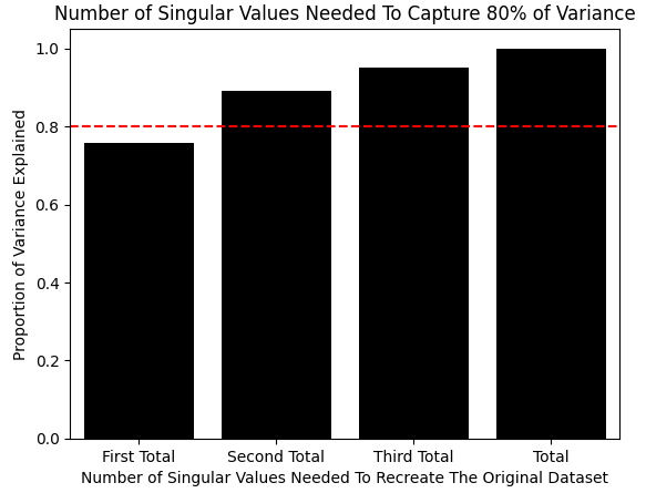
Figure 2: We only require the first 2 principal components to capture 80% of the variation observed in the dataset
We can also inspect the correlations between strategy returns. Notably, the Moving Average and RSI strategies show strong positive correlation, which may offer exploitable insight.
data.iloc[:,-12:-8].corr()
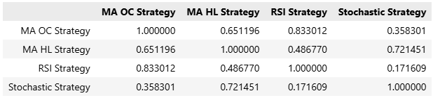
Figure 3: Visualizing the correlation matrix of the market data inputs we have available
Having identified the dominant principal components, we still need to determine which strategies contribute positively to each. These contributions are known as principal component loadings. We focus on strategies with positive loadings on the dominant components, as they are expected to perform well when the market exhibits the corresponding behavior.
VT
array([[ 0.64587337, 0.37029478, 0.63092801, 0.21830991],
[ 0.10444288, -0.33948578, 0.38679319, -0.85101828],
[ 0.64575265, 0.19765237, -0.67157641, -0.30483139],
[ 0.39362773, -0.84176287, -0.03613857, 0.36767716]])
Finally, we plot the strategy returns generated by these selected combinations in Figure 4.
plt.plot(data.iloc[:,13]+data.iloc[:,14]+data.iloc[:,15]+data.iloc[:,16],color='red')
plt.plot(data.iloc[:,13]+data.iloc[:,15],color='Orange')
plt.plot(data.iloc[:,13]+data.iloc[:,14],color='Green')
plt.plot(data.iloc[:,13]+data.iloc[:,16],color='Blue')
plt.legend(['High Risk','Medium Risk','Low Risk','Minimal Risk'])
plt.grid()
plt.title('Estimating The Returns Produced by Each of Our Risk Settings')
plt.ylabel('Estimated Profit')
plt.xlabel('Historical Epochs')

Figure 4: Visualzing the new streams of returns suggested to us by the SVD factorization
Implementing Our Strategy in MQL5
We are now ready to implement our trading application in MQL5. As is standard in our articles, we begin by defining system constants to ensure the application behaves consistently with the expectations set during the modeling phase. //+------------------------------------------------------------------+ //| Automatic Strategy Selection.mq5 | //| Gamuchirai Ndawana | //| https://www.mql5.com/en/users/gamuchiraindawa | //+------------------------------------------------------------------+ #property copyright "Gamuchirai Ndawana" #property link "https://www.mql5.com/en/users/gamuchiraindawa" #property version "1.00" //+------------------------------------------------------------------+ //| System definiyions | //+------------------------------------------------------------------+ #define MA_PERIOD 5 //--- Moving Average Period #define MA_TYPE MODE_SMA //--- Type of moving average #define RSI_PERIOD 15 //--- RSI Period #define STOCH_K 5 //--- Stochastich K Period #define STOCH_D 3 //--- Stochastich D Period #define STOCH_SLOWING 3 //--- Stochastic slowing #define STOCH_MODE MODE_EMA //--- Stochastic mode #define STOCH_PRICE STO_LOWHIGH //--- Stochastic price feeds #define TOTAL_STRATEGIES 4 //--- Total strategies we have to choose from
Next, we load the trade library to manage market positions and define the global variables used throughout the application’s lifecycle.
//+------------------------------------------------------------------+
//| System libraries                                                 |
//+------------------------------------------------------------------+
#include <Trade\Trade.mqh>
CTrade Trade;
First, we set up variables for our technical indicators and their outputs. Then, we define Mql objects to store time and tick data. Finally, we declare arrays to hold principal component weights—recall that strategies with positive responses to identified modes were assigned a weight of 1, and others a weight of 0.
//+------------------------------------------------------------------+
//| Global variables                                                 |
//+------------------------------------------------------------------+
int ma_c_handle,ma_o_handle,ma_h_handle,ma_l_handle,rsi_handle,stoch_handle,atr_handle;
double ma_c_reading[],ma_o_reading[],ma_h_reading[],ma_l_reading[],rsi_reading[],sto_reading_main[],sto_reading_signal[],atr_reading[];
double long_vote,short_vote;

MqlDateTime ts,tc;
MqlTick     current_tick;

double const weights_1 [] = {1,1,1,1};
double const weights_2 [] = {1,0,1,0};
double const weights_3 [] = {1,1,0,0};
double const weights_4 [] = {1,0,0,1};
double selected_weights[] = {0,0,0,0};
We then define a custom enumeration that allows the user to select which mode the application should operate under. Since we aim to explore new strategies, it’s easier to test the four strategies suggested by SVD than to manually evaluate every possible combination.
//+------------------------------------------------------------------+
//| Custom enumrations                                               |
//+------------------------------------------------------------------+
enum operation_modes
  {
   HIGH=0,     //High Risk
   MID=1,      //Medium Risk
   LOW=2,      //Low Risk
   MINIMUM=3   //Minimum Risk
  };
We also define an input parameter that lets us sweep over these four strategy configurations.
//+------------------------------------------------------------------+
//| User inputs                                                      |
//+------------------------------------------------------------------+
input group "User Risk Settings"
input operation_modes  user_mode = 1;//Define Your Risk Settings
When the application starts, we use a `switch` statement to load the user-selected weights into the weights array (initialized with zeros). We then set up time and technical indicators accordingly.
//+------------------------------------------------------------------+
//| Expert initialization function                                   |
//+------------------------------------------------------------------+
int OnInit()
  {
//--- Setup our risk settings
   switch(user_mode)
     {
      case(0):
         Print("High risk mode selected");
         ArrayCopy(selected_weights,weights_1,0,0,WHOLE_ARRAY);
         break;
      case(1):
         Print("Medium risk mode selected");
         ArrayCopy(selected_weights,weights_2,0,0,WHOLE_ARRAY);
         break;
      case(2):
         Print("Low risk mode selected");
         ArrayCopy(selected_weights,weights_3,0,0,WHOLE_ARRAY);
         break;
      case(3):
         Print("Minimum risk mode selected");
         ArrayCopy(selected_weights,weights_4,0,0,WHOLE_ARRAY);
         break;
      default:
         Print("No risk mode selected! No Trades will be placed");
         break;
     }

//--- Setup the time
   TimeLocal(tc);
   TimeLocal(ts);

//---Setup our technical indicators
   ma_c_handle = iMA(_Symbol,PERIOD_CURRENT,MA_PERIOD,0,MA_TYPE,PRICE_CLOSE);
   ma_o_handle = iMA(_Symbol,PERIOD_CURRENT,MA_PERIOD,0,MA_TYPE,PRICE_OPEN);
   ma_h_handle = iMA(_Symbol,PERIOD_CURRENT,MA_PERIOD,0,MA_TYPE,PRICE_HIGH);
   ma_l_handle = iMA(_Symbol,PERIOD_CURRENT,MA_PERIOD,0,MA_TYPE,PRICE_LOW);
   atr_handle = iATR(_Symbol,PERIOD_CURRENT,14);
   rsi_handle  = iRSI(_Symbol,PERIOD_CURRENT,RSI_PERIOD,PRICE_CLOSE);
   stoch_handle = iStochastic(_Symbol,PERIOD_CURRENT,STOCH_K,STOCH_D,STOCH_SLOWING,STOCH_MODE,STOCH_PRICE);
//---
   return(INIT_SUCCEEDED);
  }
When the application is no longer in use, we release any technical indicators we allocated.
//+------------------------------------------------------------------+
//| Expert deinitialization function                                 |
//+------------------------------------------------------------------+
void OnDeinit(const int reason)
  {
//---
   IndicatorRelease(ma_c_handle);
   IndicatorRelease(ma_o_handle);
   IndicatorRelease(ma_h_handle);
   IndicatorRelease(ma_l_handle);
   IndicatorRelease(rsi_handle);
   IndicatorRelease(stoch_handle);
   IndicatorRelease(atr_handle);
  }
When new price data arrives and a new day starts, we update the time and indicator readings. If no positions are open, the system holds a vote among all strategies with a weight of 1. The majority vote determines whether a long or short entry is taken.
//+------------------------------------------------------------------+
//| Expert tick function                                             |
//+------------------------------------------------------------------+
void OnTick()
  {
//---
   TimeLocal(ts);

   if(ts.day != tc.day)
     {
      //--- Update the time
      TimeLocal(tc);

      //--- Update Our indicator readings
      CopyBuffer(ma_c_handle,0,0,1,ma_c_reading);
      CopyBuffer(ma_o_handle,0,0,1,ma_o_reading);
      CopyBuffer(ma_h_handle,0,0,1,ma_h_reading);
      CopyBuffer(ma_l_handle,0,0,1,ma_l_reading);
      CopyBuffer(rsi_handle,0,0,1,rsi_reading);
      CopyBuffer(stoch_handle,0,0,1,sto_reading_main);
      CopyBuffer(stoch_handle,0,0,1,sto_reading_signal);
      CopyBuffer(atr_handle,0,0,1,atr_reading);

      //--- Copy Market Data
      double close = iClose(Symbol(),PERIOD_CURRENT,0);
      SymbolInfoTick(Symbol(),current_tick);

      //--- Place a position
      if(PositionsTotal() ==0)
        {
         //--- Our strategies will vote on what should be done
         long_vote = 0;
         short_vote = 0;

         for(int i =0; i<TOTAL_STRATEGIES;i++)
           {
            //--- Is the strategy's vote valid?
            if(selected_weights[i] > 0)
              {
               //--- Moving average open close strategy
               if(i == 0)
                 {
                  if(ma_o_reading[0] > ma_c_reading[0])
                     long_vote  += selected_weights[0];

                  else
                     if(ma_o_reading[0] < ma_c_reading[0])
                        short_vote += selected_weights[0];
                 }

               //--- Moving average high low strategy
               if(i == 1)
                 {
                  if(close > ma_h_reading[0])
                     long_vote += selected_weights[1];

                  else
                     if(close < ma_l_reading[0])
                        short_vote += selected_weights[1];
                 }

               //--- RSI Strategy
               if(i == 2)
                 {
                  if(rsi_reading[0] > 50)
                     long_vote += selected_weights[2];

                  else
                     if(rsi_reading[0] < 50)
                        short_vote += selected_weights[2];

                  //--- Stochastic Strategy
                  if(i == 3)
                    {
                     if(sto_reading_main[0] > 50)
                        long_vote += selected_weights[3];

                     else
                        if(sto_reading_main[0] < 50)
                           short_vote += selected_weights[3];
                    }
                 }
              }
           }
         if(long_vote > short_vote)
            Trade.Buy(0.01,Symbol(),current_tick.ask,current_tick.ask-(1.5*atr_reading[0]),current_tick.ask+(1.5*atr_reading[0]));

         if(long_vote < short_vote)
            Trade.Sell(0.01,Symbol(),current_tick.bid,current_tick.bid+(1.5*atr_reading[0]),current_tick.bid-(1.5*atr_reading[0]));
        }

     }
  }
//+------------------------------------------------------------------+
At the end of the application, we undefine all system constants that are no longer needed.
//+------------------------------------------------------------------+
//| Undefine system constants                                        |
//+------------------------------------------------------------------+
#undef MA_PERIOD
#undef MA_TYPE
#undef RSI_PERIOD
#undef STOCH_K
#undef STOCH_D
#undef STOCH_SLOWING
#undef STOCH_MODE
#undef STOCH_PRICE
#undef TOTAL_STRATEGIES
//+------------------------------------------------------------------+
Analyzing Our Results
We can now analyze the results of our application. First, we select date ranges outside the historical data used for model development.
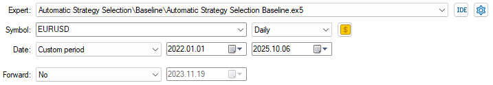
Figure 5: Selecting the back test days for our baseline version of the trading application
Next, we configure the modeling to use real ticks with random delay to emulate real market conditions.
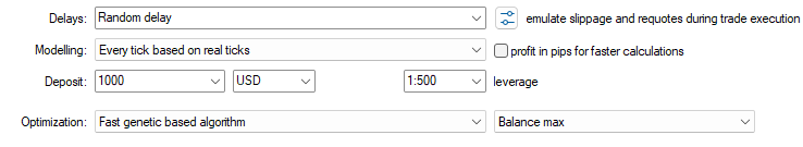
Figure 6: Selecting 'Random delay' settings will ensure that our back test will emulate real market coniditons
Then we specify the inputs to search over. Since we only have four candidate strategies, we let the genetic optimizer perform a line search over these four inputs.

Figure 7: Selecting the minimum and maximum value we will let the genetic optimizer search over
In Figure 8, we see that the first two strategies suggested by SVD were profitable, while the remaining two were unreliable. Recall from Figure 2 that these same two principal components accounted for over 80% of the variation in the training data. This suggests that the market is driven by two stable modes of behavior, while the others are weak and unstable.
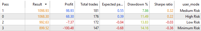
Figure 8: Analyzing the results from our historical back test of market data
Improving Our Results
Let us now turn to our second, black-box solution. This approach seeks to identify the optimal strategy based on current market conditions.
import onnx
from sklearn.linear_model import Ridge
from sklearn.neural_network import MLPRegressor
from skl2onnx.convert import convert_sklearn
from skl2onnx.common.data_types import FloatTensorType
from sklearn.model_selection import RandomizedSearchCV,TimeSeriesSplit
We begin by loading the necessary libraries and defining a custom time series validation object to apply cross-validation carefully when training deep neural networks.
tscv = TimeSeriesSplit(n_splits=5,gap=HORIZON)Next, we specify the neural network parameters to search over. Since the parameter space is large, we only explore a subset that we expect to contain a potential solution. This makes configuration more challenging than in our white-box approach.
dist = {
    'max_iter':[10,50,100,500,1000,5000,10000,50000,100000],
    'activation':['tanh','relu','identity','logistic'],
    'alpha':[10e0,10e-1,10e-2,10e-3,10e-4,10-5,10e-6],
    'solver':['lbfgs','adam','sgd'],
    'learning_rate':['constant','invscaling','adaptive'],
    'hidden_layer_sizes':[(11,1),(11,11),(11,11,11),(11,11,11,11),(11,22,33,44),(11,22,55,22,11),(11,100,11),(11,5,2,5,11),(11,3,9,18,9,3)]
}
We then define the basic neural network parameters that remain fixed across experiments.
model = MLPRegressor(shuffle=False,early_stopping=False,random_state=0,verbose=True)
With configuration complete, we perform the search for optimal parameters. Note the importance of the `n_iter` parameter in randomized search—more iterations typically improve search quality.
rscv = RandomizedSearchCV(model,dist,random_state=0,n_iter=20,scoring='neg_mean_squared_error',cv=tscv,n_jobs=-1,refit=True)
Begin the search.
res = rscv.fit(X,y)
Iteration 1, loss = 0.21844802
Iteration 2, loss = 0.13287107
Iteration 3, loss = 0.08159530
Iteration 4, loss = 0.07053761
Iteration 5, loss = 0.07051259
Once the search is complete, the best model is stored in the `best_estimator_` attribute.
res.best_estimator_

Figure 9: The optimal neural network found by randomized search procedure during the iterations we allowed for our discussion
Before exporting to ONNX, we define the input and output shape of our neural network.
initial_types = [('float_input',FloatTensorType([1,X.shape[1]]))]
final_types   = [('float_output',FloatTensorType([y.shape[1],1]))]
Next, save the model as an ONNX prototype.
onnx_proto = convert_sklearn(model=res.best_estimator_,initial_types=initial_types,final_types=final_types,target_opset=12)Write the ONNX model to disk with the `.onnx` extension.
onnx.save(onnx_proto,'Unsupervised Strategy Selection MLP.onnx')
Implementing Our Improvements
We now load the ONNX model.
//+------------------------------------------------------------------+
//| System resources                                                 |
//+------------------------------------------------------------------+
#resource "\\Files\\USS\\Unsupervised Strategy Selection MLP.onnx" as const uchar onnx_buffer[];
Define the input and output shapes of the ONNX model.
#define ONNX_INPUTS 11                     //--- Total inputs needed by our ONNX model
#define ONNX_OUTPUTS 8                     //--- Total outputs needed by our ONNX model
A few additional global variables are required to handle the model’s inputs and outputs.
long onnx_model;
vectorf onnx_features,onnx_targets;
During application initialization, we load the ONNX model from the buffer and set its input and output shapes as defined in Python. After verifying these and ensuring the model is valid, we proceed.
//+------------------------------------------------------------------+
//| Expert initialization function                                   |
//+------------------------------------------------------------------+
int OnInit()
  {

//--- Prepare the model's inputs and outputs
   onnx_features = vectorf::Zeros(ONNX_INPUTS);
   onnx_targets  = vectorf::Zeros(ONNX_OUTPUTS);

//--- Create the ONNX model
   onnx_model = OnnxCreateFromBuffer(onnx_buffer,ONNX_DATA_TYPE_FLOAT);

//--- Define the I/O shape
   ulong input_shape[] = {1,ONNX_INPUTS};
   ulong output_shape[] = {ONNX_OUTPUTS,1};

   if(!OnnxSetInputShape(onnx_model,0,input_shape))
     {
      Print("Failed to define ONNX input shape");
      return(INIT_FAILED);
     }

   if(!OnnxSetOutputShape(onnx_model,0,output_shape))
     {
      Print("Failed to define ONNX output shape");
      return(INIT_FAILED);
     }

//--- Check if the model is valid
   if(onnx_model == INVALID_HANDLE)
     {
      Print("Failed to create our ONNX model from buffer");
      return(INIT_FAILED);
     }

//--- Setup the time
   TimeLocal(tc);
   TimeLocal(ts);

//---Setup our technical indicators
   ma_c_handle = iMA(_Symbol,PERIOD_CURRENT,MA_PERIOD,0,MA_TYPE,PRICE_CLOSE);
   ma_o_handle = iMA(_Symbol,PERIOD_CURRENT,MA_PERIOD,0,MA_TYPE,PRICE_OPEN);
   ma_h_handle = iMA(_Symbol,PERIOD_CURRENT,MA_PERIOD,0,MA_TYPE,PRICE_HIGH);
   ma_l_handle = iMA(_Symbol,PERIOD_CURRENT,MA_PERIOD,0,MA_TYPE,PRICE_LOW);
   atr_handle = iATR(_Symbol,PERIOD_CURRENT,14);
   rsi_handle  = iRSI(_Symbol,PERIOD_CURRENT,RSI_PERIOD,PRICE_CLOSE);
   stoch_handle = iStochastic(_Symbol,PERIOD_CURRENT,STOCH_K,STOCH_D,STOCH_SLOWING,STOCH_MODE,STOCH_PRICE);
//---
   return(INIT_SUCCEEDED);
  }
When the ONNX model is no longer needed, we release it and free its resources.
//+------------------------------------------------------------------+
//| Expert deinitialization function                                 |
//+------------------------------------------------------------------+
void OnDeinit(const int reason)
  {
//---
   OnnxRelease(onnx_model);
  }
When new price levels are received, we update our indicator buffers and cast all inputs to float, as required by ONNX. The model predicts the anticipated cumulative return two steps ahead, so we check whether the slope of the cumulative balance is positive. If so, we place trades aligned with the strategy that exhibits the largest expected slope.
//+------------------------------------------------------------------+
//| Expert tick function                                             |
//+------------------------------------------------------------------+
void OnTick()
  {
//---
   TimeLocal(ts);

   if(ts.day != tc.day)
     {
      //--- Update the time
      TimeLocal(tc);

      //--- Update Our indicator readings
      CopyBuffer(ma_c_handle,0,0,1,ma_c_reading);
      CopyBuffer(ma_o_handle,0,0,1,ma_o_reading);
      CopyBuffer(ma_h_handle,0,0,1,ma_h_reading);
      CopyBuffer(ma_l_handle,0,0,1,ma_l_reading);
      CopyBuffer(rsi_handle,0,0,1,rsi_reading);
      CopyBuffer(stoch_handle,0,0,1,sto_reading_main);
      CopyBuffer(stoch_handle,0,0,1,sto_reading_signal);
      CopyBuffer(atr_handle,0,0,1,atr_reading);

      //--- Set our model inputs
      onnx_features[0] = (float) iOpen(Symbol(),PERIOD_CURRENT,0);
      onnx_features[1] = (float) iHigh(Symbol(),PERIOD_CURRENT,0);
      onnx_features[2] = (float) iLow(Symbol(),PERIOD_CURRENT,0);
      onnx_features[3] = (float) iClose(Symbol(),PERIOD_CURRENT,0);
      onnx_features[4] = (float) ma_o_reading[0];
      onnx_features[5] = (float) ma_h_reading[0];
      onnx_features[6] = (float) ma_l_reading[0];
      onnx_features[7] = (float) ma_c_reading[0];
      onnx_features[8] = (float) rsi_reading[0];
      onnx_features[9] = (float)  sto_reading_main[0];
      onnx_features[10] = (float) sto_reading_signal[0];

      //--- Copy Market Data
      double close = iClose(Symbol(),PERIOD_CURRENT,0);
      SymbolInfoTick(Symbol(),current_tick);

      //--- Place a position
      if(PositionsTotal() ==0)
        {
         if(OnnxRun(onnx_model,ONNX_DATA_TYPE_FLOAT,onnx_features,onnx_targets))
           {
            Comment("Onnx Model Prediction: \n",onnx_targets);

            //--- Store our result
            vectorf res = {onnx_targets[1]-onnx_targets[0],onnx_targets[3]-onnx_targets[2],onnx_targets[5]-onnx_targets[4],onnx_targets[7]-onnx_targets[6]};

            if(res.Max() > 0)
              {
               Print("Trading oppurtunity found");
               Print(res);
               if(res.ArgMax()==0)
                 {
                  if(ma_o_reading[0]<ma_c_reading[0])
                     Buy();

                  if(ma_o_reading[0]>ma_c_reading[0])
                     Sell();
                 }

               if(res.ArgMax()==1)
                 {
                  if(close>ma_h_reading[0])
                     Buy();

                  if(close<ma_l_reading[0])
                     Sell();
                 }


               if(res.ArgMax()==2)
                 {
                  if(rsi_reading[0]>50)
                     Buy();

                  if(rsi_reading[0]<50)
                     Sell();
                 }

               if(res.ArgMax()==3)
                 {
                  if(sto_reading_main[0]>50)
                     Buy();


                  if(sto_reading_main[0]<50)
                     Sell();
                 }
              }
            else
              {
               Print("No trading oppurtunities expected.");
              }
           }
        }
     }
  }
//+------------------------------------------------------------------+
Finally, for maintainability, we define separate methods for entering long and short positions, avoiding repetition in our code.
//+------------------------------------------------------------------+
//| Enter a long position                                            |
//+------------------------------------------------------------------+
void Buy(void)
  {
   Trade.Buy(0.01,Symbol(),current_tick.ask,current_tick.ask-(1.5*atr_reading[0]),current_tick.ask+(1.5*atr_reading[0]));
  }

//+------------------------------------------------------------------+
//| Enter a short position                                           |
//+------------------------------------------------------------------+
void Sell(void)
  {
   Trade.Sell(0.01,Symbol(),current_tick.bid,current_tick.bid+(1.5*atr_reading[0]),current_tick.bid-(1.5*atr_reading[0]));
  }
//+------------------------------------------------------------------+
We are now ready to backtest the black-box version of our trading application.
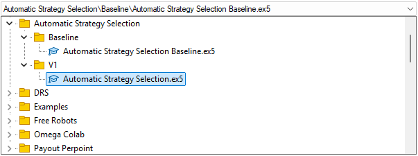
Figure 10: Select the right version of the application for our second test
Start by selecting the correct version of the application and loading the appropriate test dates—these must remain consistent with the rest of our discussion.
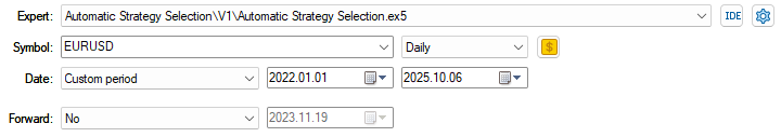
Figure 11: Be sure you have carefully identified the right backtesting dates that we will use for our test
The equity curve shows the positive account balance trend we expected. However, recall that the strategy was selected automatically—the deep neural network chose the single strategy it deemed optimal.

Figure 12: The equity curve produced by the trading strategy we are following suggests to us that our black-box solution grasped the task at hand
Upon reviewing the performance statistics, we see that the black-box approach underperformed relative to the white-box solution. This outcome was expected, given the black-box setup was more time-consuming and could likely improve with a greater number of search iterations.

Figure 14: The detailed results produced by our black-box solution
Conclusion
In conclusion, this article demonstrated how to automatically identify trading strategies using the MetaTrader 5 toolkit. We showed how a computer can rapidly uncover strategies that might otherwise escape human detection—the data reveals patterns whether we see them or not. Our discussion highlighted the advantages of white-box solutions driven by unsupervised matrix factorization: they require less configuration time, offer clearer interpretability, and provide explicit guidance on which strategies to retain, ultimately saving time and adding diagnostic value. In contrast, black-box solutions become more valuable in complex market conditions where white-box approaches may fall short.
| File Name | File Description |
|---|---|
| Automatic Strategy Selection Baseline.mq5 | Our white-box solution of 4 unique strategies generated by the SVD factorization. |
| Automatic Strategy Selection.mq5 | Our black-box solution generated by our deep neural network of the EURUSD market. |
| Fetch Data Indicators.mq5 | The MQL5 script we built to fetch the market data we need and begin our analysis of strategy returns. |
Warning: All rights to these materials are reserved by MetaQuotes Ltd. Copying or reprinting of these materials in whole or in part is prohibited.
This article was written by a user of the site and reflects their personal views. MetaQuotes Ltd is not responsible for the accuracy of the information presented, nor for any consequences resulting from the use of the solutions, strategies or recommendations described.

- Free trading apps
- Over 8,000 signals for copying
- Economic news for exploring financial markets
You agree to website policy and terms of use