Self Optimizing Expert Advisors in MQL5 (Part 17): Ensemble Intelligence

All algorithmic trading strategies are difficult to set up and maintain, regardless of their complexity. This universal problem is shared by beginners and experts alike. Beginners struggle to keep tuning the periods of their moving average crossover strategies, while experts are just as restless adjusting the weights of their deep neural networks. There are material problems on either side of the fence.

Machine learning models are fragile and often fall apart in live trading environments. Their opaque and complex designs make them even harder to troubleshoot and diagnose for performance bottlenecks. On the otherhand, human strategies can be more resilient but often require manual configuration to get started—an intensive process depending on the approach. This article proposes an ensemble framework in which supervised models and human intuition build on each other to overcome their collective limitations in an accelerated way.

To attain this end, we designed our strategy and statistical model to share the same four technical indicators. We selected a moving average channel strategy and fit a Ridge Regression model on those same indicators. Doing this, allowed us to quickly identify a profitable configuration for the entire system.

The technical indicators give us centralized control over both human intuition and the supervised model. Requiring the strategy to open positions only when both the traditional and statistical components agreed produced a profitable outcome from two independently unprofitable systems. This is the motivation behind our ensemble framework: our strategies appear to consistently correct each other faster than we can equivalently correct either one.

Our approach allows the statistical model to learn from the same technical indicators used by the strategy, making ensemble stacking more practical and helping us find stable configurations that would otherwise be time-consuming to establish. This centralized control means we only need to configure a few technical indicators that affect both components—allowing us to quickly discover which moving averages matter, regardless of their underlying periods. No tuning of moving average periods was necessary, even though the article will establish that the initial strategy was unprofitable with the selected periods that we kept for demonstratitve purposes. The system learns to correct itself.

Visualizing The Trading Strategy

The strategy relies on two moving average indicators, one placed on the high and low price feeds respectively. The indicators form a channel, with the space between them depending on the given volatility of the market. An illustration of the strategy is provided in Figure 1 below. The strategy provides long signals when price levels break above the uppermost channel, and the converse holds true for sell signals. In the white box in the top right corner of Figure 1, we can observe that the strategy generated two opposing signals in a short space of time; the strategy has visible levels of noise.

Figure 1: Identifying a trading oppurtunity according to the moving average channel strategy

While the strategy is noisy, it serves as a reliable guide to the overall trend in the market.

Figure 2: Though the strategy has noise, it appears sound overall

Establishing A Baseline Performance Level

To get started, we will first define system constants that we will keep fixed throughout our test. 

//+------------------------------------------------------------------+
//|                                                           EI.mq5 |
//|                                               Gamuchirai Ndawana |
//|                    https://www.mql5.com/en/users/gamuchiraindawa |
//+------------------------------------------------------------------+
#property copyright "Gamuchirai Ndawana"
#property link      "https://www.mql5.com/en/users/gamuchiraindawa"
#property version   "1.00"

//+------------------------------------------------------------------+
//| System constants                                                 |
//+------------------------------------------------------------------+
#define SYSTEM_TF PERIOD_D1
#define MA_SHIFT 0
#define MA_TYPE MODE_EMA
#define ATR_PERIOD 14
#define PADDING 2

Next, we will load a few helper libraries we need for our exercise.

//+------------------------------------------------------------------+
//| Libraries                                                        |
//+------------------------------------------------------------------+
#include <Trade\Trade.mqh>
#include <VolatilityDoctor\Trade\TradeInfo.mqh>

CTrade Trade;
TradeInfo *TradeHelper;

Global variables are needed in almost all applications, we need them to keep track of our technical indicator readings and time.

//+------------------------------------------------------------------+
//| Define global variables                                          |
//+------------------------------------------------------------------+
int    ma_h_handler,ma_l_handler,atr_handler;
double ma_h[],ma_l[],atr[];
MqlDateTime tc,ts;

We will define an input value of 20, if you change this value, remember to keep the change consistent in the script.

//+------------------------------------------------------------------+
//| Input varaibles                                                  |
//+------------------------------------------------------------------+
input group "Technical Indicators"
input int MA_PERIOD = 20;//Moving average period

When our application is initialized, we will load the technical indicators we need, and create new instances of the class instances we need.

//+------------------------------------------------------------------+
//| Expert initialization function                                   |
//+------------------------------------------------------------------+
int OnInit()
  {
//--- Setup our technical indicators
   ma_h_handler = iMA(Symbol(),SYSTEM_TF,MA_PERIOD,MA_SHIFT,MA_TYPE,PRICE_HIGH);
   ma_l_handler = iMA(Symbol(),SYSTEM_TF,MA_PERIOD,MA_SHIFT,MA_TYPE,PRICE_LOW);
   atr_handler = iATR(Symbol(),SYSTEM_TF,ATR_PERIOD);
   TradeHelper = new TradeInfo(Symbol(),SYSTEM_TF);

//--- Mark the time
   TimeLocal(tc);
   TimeLocal(ts);
//---
   return(INIT_SUCCEEDED);
  }

If our application is no longer in use, we will release the technical indicators we are no longer using.

//+------------------------------------------------------------------+
//| Expert deinitialization function                                 |
//+------------------------------------------------------------------+
void OnDeinit(const int reason)
  {
//---
   delete TradeHelper;
   IndicatorRelease(ma_h_handler);
   IndicatorRelease(ma_l_handler);
   IndicatorRelease(atr_handler);
  }

Our application will perform routine tasks each hour. This is done by checking for the passage of time using the specialized MqlDateTime object. Then we proceed to update the technical indicator buffers and store the current close price. Finally, we perform a check for the trading signal: if the close price has broken out of the moving average channel, we enter positions to reflect confidence in the move.

//+------------------------------------------------------------------+
//| Expert tick function                                             |
//+------------------------------------------------------------------+
void OnTick()
  {
//---
   TimeLocal(ts);

   if(ts.hour != tc.hour)
     {
      if(PositionsTotal()==0)
        {
         //--- Update the time
         TimeLocal(tc);

         //--- Update the indicator buffer
         CopyBuffer(ma_h_handler,0,0,1,ma_h);
         CopyBuffer(ma_l_handler,0,0,1,ma_l);
         CopyBuffer(atr_handler,0,0,1,atr);

         //--- Check if the current price is above or below the channel
         double c = iClose(Symbol(),SYSTEM_TF,0);

         if(c > ma_h[0])
            Trade.Buy(TradeHelper.MinVolume(),Symbol(),TradeHelper.GetAsk(),TradeHelper.GetBid()-(atr[0]*PADDING),TradeHelper.GetBid()+(atr[0]*PADDING));

         else
            if(c < ma_l[0])
               Trade.Sell(TradeHelper.MinVolume(),Symbol(),TradeHelper.GetBid(),TradeHelper.GetAsk()+(atr[0]*PADDING),TradeHelper.GetAsk()-(atr[0]*PADDING));
        }
     }
  }
//+------------------------------------------------------------------+

Finally, we undefine all system constants we defined earlier.

//+------------------------------------------------------------------+
//| Undefine system constants                                        |
//+------------------------------------------------------------------+
#undef SYSTEM_TF
#undef MA_SHIFT
#undef MA_TYPE
#undef ATR_PERIOD
#undef PADDING

Load the benchmark application and set our test dates accordingly. We have selected more than three years of daily EURUSD data for this exercise, spanning from January 2022 to January 2025.

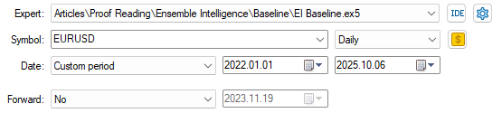
Figure 3: Selecting the dates our application to establish a baseline performance over

A combination of random delay and modeling based on real-tick settings ensures the best results and parallels live trading.

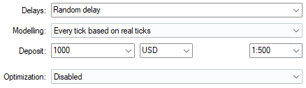
Figure 4: Selecting the test conditions we want to test our application on

We have also allowed the user to specify their own period and play an active role in reading. Otherwise, the value of 20 was selected arbitrarily.

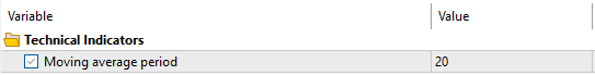
Figure 5: Our current exercise allows us to pick arbitrary periods for assessment

As explained in the introduction, the value of 20 was not profitable. However, as we shall see, our statistical strategy can learn from this and help us correctly filter out noise without always having to sweep for different periods for our technical indicators.

Figure 6: The equity curve producedx by our trading application has no stability and gives us little confidence

The benchmark results we have produced are in line with the equity curve we observed earlier—negative, and normally a sign we should abandon our idea—but for today, we will proceed with the system intact.

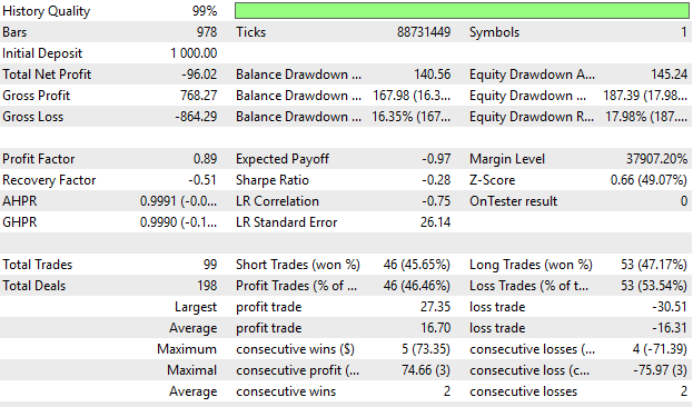
Figure 7: The detailed statistics we have with our benchmark application show us we can still improve

Fetch Historical Market Data

Now let us build a script to fetch historical market data and write it out to CSV. We will use this data to help us build a statistical strategy around the EURUSD market.

//+------------------------------------------------------------------+
//|                                                      ProjectName |
//|                                      Copyright 2020, CompanyName |
//|                                       http://www.companyname.net |
//+------------------------------------------------------------------+
#property copyright "Copyright 2024, MetaQuotes Ltd."
#property link      "https://www.mql5.com"
#property version   "1.00"
#property script_show_inputs

//--- Define our moving average indicator
#define MA_PERIOD 5                 //--- Moving Average Period
#define MA_TYPE   MODE_SMA          //--- Type of moving average we have
#define HORIZON   5                 //--- Forecast horizon

//--- Our handlers for our indicators
int ma_handle,ma_o_handle,ma_h_handle,ma_l_handle;

//--- Data structures to store the readings from our indicators
double ma_reading[],ma_o_reading[],ma_h_reading[],ma_l_reading[];

//--- File name
string file_name = Symbol() + " Detailed Market Data As Series Moving Average.csv";

//--- Amount of data requested
input int size = 3000;

//+------------------------------------------------------------------+
//| Our script execution                                             |
//+------------------------------------------------------------------+
void OnStart()
  {
   int fetch = size + (HORIZON * 2);
//---Setup our technical indicators
   ma_handle = iMA(_Symbol,PERIOD_CURRENT,MA_PERIOD,0,MA_TYPE,PRICE_CLOSE);
   ma_o_handle = iMA(_Symbol,PERIOD_CURRENT,MA_PERIOD,0,MA_TYPE,PRICE_OPEN);
   ma_h_handle = iMA(_Symbol,PERIOD_CURRENT,MA_PERIOD,0,MA_TYPE,PRICE_HIGH);
   ma_l_handle = iMA(_Symbol,PERIOD_CURRENT,MA_PERIOD,0,MA_TYPE,PRICE_LOW);

//---Set the values as series
   CopyBuffer(ma_handle,0,0,fetch,ma_reading);
   ArraySetAsSeries(ma_reading,true);
   CopyBuffer(ma_o_handle,0,0,fetch,ma_o_reading);
   ArraySetAsSeries(ma_o_reading,true);
   CopyBuffer(ma_h_handle,0,0,fetch,ma_h_reading);
   ArraySetAsSeries(ma_h_reading,true);
   CopyBuffer(ma_l_handle,0,0,fetch,ma_l_reading);
   ArraySetAsSeries(ma_l_reading,true);

//---Write to file
   int file_handle=FileOpen(file_name,FILE_WRITE|FILE_ANSI|FILE_CSV,",");

   for(int i=size;i>=1;i--)
     {
      if(i == size)
        {
         FileWrite(file_handle,"Time",
                   //--- OHLC
                   "True Open",
                   "True High",
                   "True Low",
                   "True Close",
                   //--- MA OHLC
                   "True MA O",
                   "True MA H",
                   "True MA L",
                   "True MA C"
                  );
        }

      else
        {
         FileWrite(file_handle,
                   iTime(_Symbol,PERIOD_CURRENT,i),
                   //--- OHLC
                   iClose(_Symbol,PERIOD_CURRENT,i),
                   iOpen(_Symbol,PERIOD_CURRENT,i),
                   iHigh(_Symbol,PERIOD_CURRENT,i),
                   iLow(_Symbol,PERIOD_CURRENT,i),
                   //--- MA OHLC
                   ma_o_reading[i],
                   ma_h_reading[i],
                   ma_l_reading[i],
                   ma_reading[i]
                  );
        }
     }
//--- Close the file
   FileClose(file_handle);
  }
//+------------------------------------------------------------------+

//+------------------------------------------------------------------+
//| Undefine system constants                                        |
//+------------------------------------------------------------------+
#undef HORIZON
#undef MA_PERIOD
#undef MA_TYPE
//+------------------------------------------------------------------+

Analyzing Historical Market Data in Python

Load our standard Python libraries.

#Load the libraries we need
import pandas as pd
import numpy as np

Read the market data we wrote to CSV earlier.

#Read in the data
data = pd.read_csv("../EURUSD Detailed Market Data As Series Moving Average.csv")
data

Define our forecast horizon.

#Define the forecast horizon
HORIZON = 20

Drop all historical data that overlaps with the backtest period.

#Drop the dates that overlap with the back test
data = data.iloc[:-(365*3),:]
_ = data.iloc[-(365*3):,:]

Label the market data so we can model which side of the moving average the close price is expected to be on. This is what drives our strategy from the perspective of human intuition.

#Label the data
data['Target H'] = data['Close'].shift(-HORIZON) - data['MA H'].shift(-HORIZON)
data['Target L'] = data['Close'].shift(-HORIZON) - data['MA L'].shift(-HORIZON)

#Drop missing rows
data = data.iloc[:-HORIZON,:]

Load our ONNX libraries. ONNX, which stands for Open Neural Network Exchange, is an open-source library that helps us build and deploy machine learning models without carrying over dependencies from their training environments.

from sklearn.linear_model import Ridge
import onnx
from skl2onnx import convert_sklearn 
from skl2onnx.common.data_types import FloatTensorType

Fit the model on all the training data.

model = Ridge(alpha=1e-3)
model.fit(data.iloc[:,1:-2],data.loc[:,['Target H','Target L']])

Define the input and output shapes of our ONNX model.

initial_types = [('float_input',FloatTensorType([1,8]))]
final_types = [('float_output',FloatTensorType([1,2]))]

Save the ONNX model as an ONNX prototype.

onnx_proto = convert_sklearn(model=model,initial_types=initial_types,final_types=final_types,target_opset=12)

Save the ONNX prototype as a file on your drive. 

onnx.save(onnx_proto,'EURUSD MA R.onnx')

Beating The Baseline

We will now focus on the parts of our codebase that will change and omit all other parts that did not. The first change we will make is introducing two new system constant definitions linked to our ONNX model.

//+------------------------------------------------------------------+
//|                                                           EI.mq5 |
//|                                               Gamuchirai Ndawana |
//|                    https://www.mql5.com/en/users/gamuchiraindawa |
//+------------------------------------------------------------------+
#property copyright "Gamuchirai Ndawana"
#property link      "https://www.mql5.com/en/users/gamuchiraindawa"
#property version   "1.00"

//+------------------------------------------------------------------+
//| System constants                                                 |
//+------------------------------------------------------------------+
#define ONNX_FEATURES 8
#define ONNX_TARGETS 2

Now, we load our ONNX model.

//+------------------------------------------------------------------+
//| Dependencies                                                     |
//+------------------------------------------------------------------+
#resource "\\Files\\EURUSD MA R.onnx" as const uchar onnx_buffer[];

Now we create our ONNX model from the buffer we defined earlier and configure the input and output shapes of our model.

//+------------------------------------------------------------------+
//| Expert initialization function                                   |
//+------------------------------------------------------------------+
int OnInit()
  {
   onnx_model = OnnxCreateFromBuffer(onnx_buffer,ONNX_DATA_TYPE_FLOAT);

   if(onnx_model == INVALID_HANDLE)
     {
      Print("Failed to create ONNX model: ",GetLastError());
      return(INIT_FAILED);
     }

   ulong input_shape[]  = {1,ONNX_FEATURES};
   ulong output_shape[] = {1,ONNX_TARGETS};

   onnx_inputs = vectorf::Zeros(ONNX_FEATURES);
   onnx_output = vectorf::Zeros(ONNX_TARGETS);

   if(!OnnxSetInputShape(onnx_model,0,input_shape))
     {
      Print("Failed to define ONNX input shape: ",GetLastError());
      return(INIT_FAILED);
     }

   if(!OnnxSetOutputShape(onnx_model,0,output_shape))
     {
      Print("Failed to define ONNX output shape: ",GetLastError());
      return(INIT_FAILED);
     }

//--- Mark the time
   TimeLocal(tc);
   TimeLocal(ts);
//---
   return(INIT_SUCCEEDED);
  }

If our application is no longer in use, we must also release the ONNX model we are no longer using.

//+------------------------------------------------------------------+
//| Expert deinitialization function                                 |
//+------------------------------------------------------------------+
void OnDeinit(const int reason)
  {
//---
   OnnxRelease(onnx_model);
  }

In addition to the previous indicator updates we defined, we also need the current market inputs for our ONNX model. Recall that our model predicts how far the close price will deviate from the moving average boundaries. Positive deviations are bullish; negative deviations are bearish.

//+------------------------------------------------------------------+
//| Expert tick function                                             |
//+------------------------------------------------------------------+
void OnTick()
  {
//---
   if(ts.hour != tc.hour)
     {
      if(PositionsTotal()==0)
        {
         onnx_inputs[0] = (float) iOpen(Symbol(),SYSTEM_TF,0);
         onnx_inputs[1] = (float) iHigh(Symbol(),SYSTEM_TF,0);
         onnx_inputs[2] = (float) iLow(Symbol(),SYSTEM_TF,0);
         onnx_inputs[3] = (float) iClose(Symbol(),SYSTEM_TF,0);
         onnx_inputs[4] = (float) ma_o[0];
         onnx_inputs[5] = (float) ma_h[0];
         onnx_inputs[6] = (float) ma_l[0];
         onnx_inputs[7] = (float) ma_c[0];

         if(OnnxRun(onnx_model,ONNX_DATA_TYPE_FLOAT,onnx_inputs,onnx_output))
           {
            //--- Check if the current price is above or below the channel
            Print("Forecast: ",onnx_output);
            double c = iClose(Symbol(),SYSTEM_TF,0);
	    
            if((c > ma_h[0]) && (onnx_output[0]>0) && (onnx_output[1]>0))
               Trade.Buy(TradeHelper.MinVolume(),Symbol(),TradeHelper.GetAsk(),TradeHelper.GetBid()-(atr[0]*PADDING),TradeHelper.GetBid()+(atr[0]*PADDING));

            else
               if((c < ma_l[0]) && (onnx_output[0]<0) && (onnx_output[1]<0))
                  Trade.Sell(TradeHelper.MinVolume(),Symbol(),TradeHelper.GetBid(),TradeHelper.GetAsk()+(atr[0]*PADDING),TradeHelper.GetAsk()-(atr[0]*PADDING));
           }

         else
           {
            Print("Failed to obtain a prediction from our ONNX model: ",GetLastError());
           }
        }
     }
  }
//+------------------------------------------------------------------+

Then undefine the new definitions we made to accommodate our ONNX model.

//+------------------------------------------------------------------+
//| Undefine system constants                                        |
//+------------------------------------------------------------------+
#undef ONNX_FEATURES
#undef ONNX_TARGETS
//+------------------------------------------------------------------+

Now we will test the new version of the application we have just built together over the same test periods.

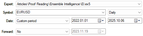
Figure 8: Then we select the same test dates we selected in our first test for consistency

As we can see, the application is still unprofitable. However, let us take a closer look at the detailed statistics.

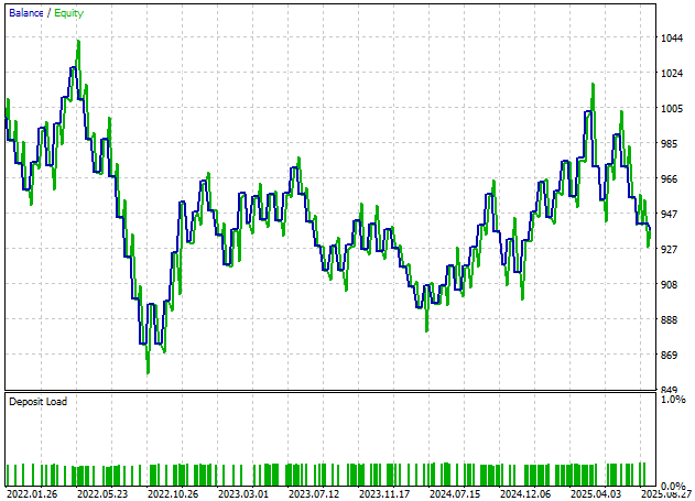
Figure 9: Our application still has not yet broken into profitability

The total net profit has increased from -$96 to -$62, but there is still plenty of room to improve.

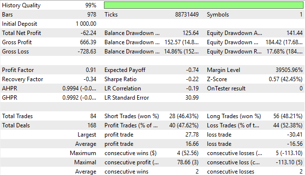
Figure 10: The detailed results of the application we have just produced still give us little confidence in the integrity of our strategy so far

Additional Improvements

Let us lean on our previous discussion of candlestick patterns to offer an alternative learning partner for our statistical strategy. These high and low price feeds are the technical inputs of our moving average indicators. We discussed the bullish engulfing candlestick in detail earlier and observed how to extract good performance from it independently of our statistical models.

if(OnnxRun(onnx_model,ONNX_DATA_TYPE_FLOAT,onnx_inputs,onnx_output))
  {
   //--- Check if the current price is above or below the channel
   Print("Forecast: ",onnx_output);
   double c = iClose(Symbol(),SYSTEM_TF,0);

   //--- Check for any bullish engulfing candle sticks
   if((onnx_output[0]>0) && (onnx_output[1]>0) && (iHigh(Symbol(),PERIOD_CURRENT,1) > iHigh(Symbol(),PERIOD_CURRENT,2)) && (iLow(Symbol(),PERIOD_CURRENT,1) < iLow(Symbol(),PERIOD_CURRENT,2)))
      Trade.Buy(TradeHelper.MinVolume(),Symbol(),TradeHelper.GetAsk(),TradeHelper.GetBid()-(atr[0]*PADDING),TradeHelper.GetBid()+(atr[0]*PADDING));
            
   //--- Check for any bearish engulfing candle sticks
   else
      if((onnx_output[0]<0) && (onnx_output[1]<0) && (iHigh(Symbol(),PERIOD_CURRENT,1) > iHigh(Symbol(),PERIOD_CURRENT,2)) && (iLow(Symbol(),PERIOD_CURRENT,1) < iLow(Symbol(),PERIOD_CURRENT,2)))
         Trade.Sell(TradeHelper.MinVolume(),Symbol(),TradeHelper.GetBid(),TradeHelper.GetAsk()+(atr[0]*PADDING),TradeHelper.GetAsk()-(atr[0]*PADDING));
  }    

Let us now repeat the test over the same periods using this revised version of our application.

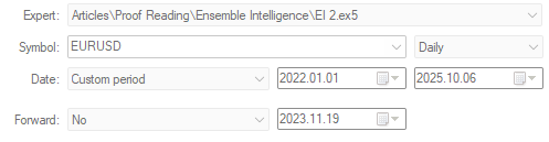
Figure 11: Running our new version of our trading strategy over the same 3 year test window

As we can see, we are now reaching new levels of profitability we could only aspire to earlier. Our application has started to gain positive momentum. But let us take a deeper look at the detailed results of this backtest.

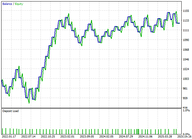
Figure 12: The equity curve produced by our new revised version of the trading application gives us measurable confidence

It is encouraging to see that our application now produces a total net profit of $126.58, though only nine short trades were placed over a three-year backtest. This is not acceptable and may indicate untapped potential we have not yet surfaced.

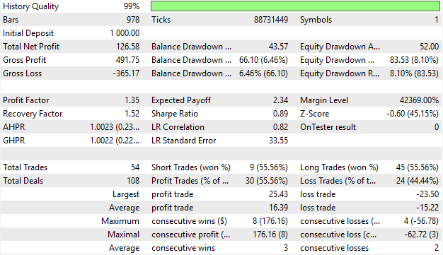
Figure 13: Analyzing detailed results produced by our improved trading strategy shows that the distribution of trades needs further refinement

Final Attempt

Let us now make our final attempt at improving the model. We will begin by making important adjustments to our model. We will forecast our technical indicators at multiple steps into the future, with each indicator modeled at one and twenty steps ahead, giving us a total of four targets.

#Label the data
data['Target H'] = data['MA H'].shift(-1)
data['Target L'] = data['MA L'].shift(-1)

data['Target H 2'] = data['MA H'].shift(-HORIZON)
data['Target L 2'] = data['MA L'].shift(-HORIZON)

#Drop missing rows
data = data.iloc[:-HORIZON,:]

We will then fit a Ridge Regression model with an alpha value of 0.001. This determines how quickly unimportant coefficients should be shrunk to zero, keeping our model focused on parameters that matter. Then we fit our model.

model = Ridge(alpha=1e-3)
model.fit(data.iloc[:,1:-4],data.loc[:,['Target H','Target L','Target H 2','Target L 2']])

The input and output shapes of the model are now defined.

initial_types = [('float_input',FloatTensorType([1,8]))]
final_types = [('float_output',FloatTensorType([1,4]))]

Finally, we will save our ONNX model to file.

onnx.save(onnx_proto,'EURUSD MA MFH R.onnx')

Implementing Our Improvements in MQL5

Now we are ready to implement our improvements in MQL5. We begin by changing the size of our ONNX model outputs.

//+------------------------------------------------------------------+
//| System constants                                                 |
//+------------------------------------------------------------------+
#define ONNX_TARGETS 4

Then we load our newly updated multi-step forecast model.

//+------------------------------------------------------------------+
//| Dependencies                                                     |
//+------------------------------------------------------------------+
#resource "\\Files\\EURUSD MA MFH R.onnx" as const uchar onnx_buffer[];

Now we can obtain a new prediction from our model and compare it against our human intuition. Whenever the close moving average is above the open, it gives us bullish sentiment about the market. On the other hand, if the ONNX model expects that both the high and low moving averages will appreciate over time, this confirms our confidence and allows us to place long positions. The opposite holds true for our sell conditions.

 if(OnnxRun(onnx_model,ONNX_DATA_TYPE_FLOAT,onnx_inputs,onnx_output))
           {
            //--- Check if the current price is above or below the channel
            Print("Forecast: ",onnx_output);
            double c = iClose(Symbol(),SYSTEM_TF,0);

            if((ma_o[0]<ma_c[0]) && (onnx_output[0]<onnx_output[2]) && (onnx_output[1]<onnx_output[3]))
               Trade.Buy(TradeHelper.MinVolume(),Symbol(),TradeHelper.GetAsk(),TradeHelper.GetBid()-(atr[0]*PADDING),TradeHelper.GetBid()+(atr[0]*PADDING));

            else
               if((ma_o[0]>ma_c[0]) && (onnx_output[0]>onnx_output[2]) && (onnx_output[1]>onnx_output[3]))
                  Trade.Sell(TradeHelper.MinVolume(),Symbol(),TradeHelper.GetBid(),TradeHelper.GetAsk()+(atr[0]*PADDING),TradeHelper.GetAsk()-(atr[0]*PADDING));
           }

Let us now test the improved version of our trading application over the same test period.

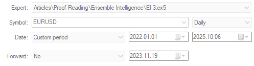
Figure 14: Testing our final configuration of our trading application over the same 3 year window we have used in this exercise

As we can see, the equity curve produced by our new application is much more resilient and shows a stronger uptrend than all earlier versions we have produced so far.

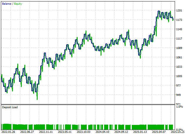
Figure 15: The equity curve produced by our final version of our trading application is reaching new highs we could not reach earlier

Additionally, our new performance levels are healthy. Our application now produces a total profit of $173.72, far better than the -$96 profit we started with, and our distribution of long and short entries is finally acceptable.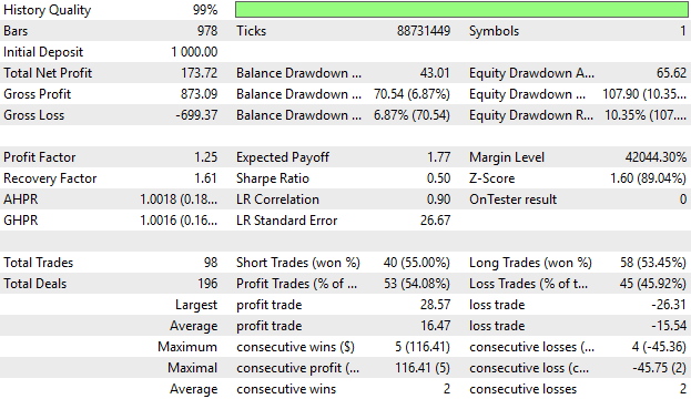

Figure 16: The detailed results produced by our refined version of the trading application gives us confidence in the changes we have made thus far

Conclusion

We have now arrived at the end of our discussion for today. This article has explored how to control the unstable nature of algorithmic trading strategies that depend on supervised models. Our solution was to build statistical models that depend on the same indicators and market data as a traditional trading strategy, and then stack the two strategies so they work as one. This procedure eliminated the need to tune parameters in the traditional strategy we started with and produced a final strategy that was more robust. Readers can easily extend this solution to integrate their favourite indicators, not just the ones illustrated in our example.

File Name	File Description
Fetch Data MA.mq5	The MQL5 script we used to fetch our historical market data from the MetaTrader 5 terminal.
EI Baseline.mq5	This application served as a profitability benchmark of the classical moving average channel strategy.
EI.mq5	Our initial attempt to outperform the benchmark, note this version of the application was not profitable.
EI 2.mq5	Our first successfull attempt to outperform the benchmark, note this version of the application was biased towards long positions.
EI 3.mq5	The best version of the moving average channel strategy we produced that both outperformed the classical strategy, and placed relatively unbiased trades.
MA Channel AI 3.ipynb	The jupyter notebook we wrote together to analyze the historical market data we fetched using our MQL5 script.