MetaTrader 5 Machine Learning Blueprint (Part 1): Data Leakage and Timestamp Fixes

Introduction

Welcome to the first instalment of our MetaTrader 5 Machine Learning Blueprint series. This article addresses a critical, yet often overlooked, issue in building robust machine learning models for financial markets using MetaTrader 5 data: the "timestamp trap." We will explore how incorrect timestamp handling can lead to insidious data leakage, compromising the integrity of your models and generating unreliable trading signals. More importantly, we will provide concrete solutions and best practices, drawing on established industry research, to ensure your data is clean, unbiased, and ready for advanced quantitative analysis.

Target Audience & Prerequisites

This article is specifically designed for quantitative traders, data scientists, and developers who possess a foundational understanding of Python, Pandas, and the MetaTrader 5 API. Familiarity with basic machine learning concepts will also be beneficial. Our goal is to equip you with the practical knowledge and tools necessary to build high-integrity datasets for developing trustworthy machine learning models in algorithmic trading.

Series Roadmap

This article marks the beginning of a comprehensive series dedicated to constructing a complete machine learning blueprint for MetaTrader 5. In this part, we lay the essential groundwork by ensuring data integrity. Future topics will delve into more advanced stages of the machine learning pipeline, including:

• Part 2 -Advanced Feature Engineering and Labelling: Techniques for defining target variables that capture true market dynamics.
• Part 3 - Model Training and Validation: Best practices for training, validating, and selecting machine learning models tailored for financial time series.
  
• Part 4 -Rigorous Back-testing and Deployment: Methodologies for evaluating model performance in realistic trading environments and strategies for deploying models live.

The MetaTrader 5 Timestamp Trap: Understanding and Prevention

Data snooping or data leakage might seem subtle, but its impact on machine learning models can be monumental—and devastating. Imagine studying for a test where you unknowingly peek at the answers beforehand. Your perfect score feels earned, but it's actually cheating. This is precisely what happens when we use MetaTrader 5's default timestamps in machine learning—data leakage unexpectedly corrupts your model's integrity.

How MetaTrader 5's Timestamps Trick You

MetaTrader 5 labels the 5-minute bar starting at 18:55, i.e., the 2nd-last bar above, as:

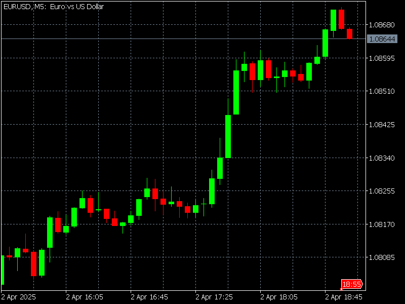
Time	Open	High	Low	Close
2 Apr 18:55	1.08718	1.08724	1.08668	1.08670

By timestamping at the start, MetaTrader 5 implies this bar's data was available at 18:55:00—a full 5 minutes before it actually closed! If your model uses this in training, it's like giving a student exam answers 5 minutes before the test begins. To counteract this, we should avoid using MetaTrader 5's precompiled time-bars, instead using tick data to create the bars we use in our models.

Why Data Leakage Matters

Data leakage can silently ruin your entire machine learning project. It happens when your model accidentally learns from information it shouldn’t have during training—like peeking into the future. As a result, the model looks incredibly accurate while training, but in reality, it’s just been fed answers it would never get in the real world.

Instead of learning genuine patterns, the model starts memorizing noise, becoming like a student who crams the answer key without understanding the material. This leads to poor performance when it’s time to make real predictions on new data.

What’s worse, a model trained with leaked data might seem trustworthy but will fail to deliver when deployed. It can give you false confidence and lead you to make bad decisions—something especially dangerous in high-stakes environments like trading, where even small mistakes can be costly.

Fixing data leakage after the fact is frustrating. It usually means going back and redoing large parts of your pipeline, wasting time, computational resources, and sometimes even money. That’s why spotting and preventing data leakage early on is so important.

Why Tick Bars Matter: A Quantitative Perspective

Financial data often arrives at irregular intervals, and for us to be able to use machine learning (ML) on it, we must regularize it, as most ML algorithms expect data in a tabular format. Those tables' rows are commonly referred to as "bars". The charts we view on MetaTrader 5, and practically all other charting platforms, represent time-bars, which convert tick data into Open, High, Low, Close and Volume columns by sampling ticks over a fixed time horizon, such as once every minute.

Although time bars are perhaps the most popular among practitioners and academics, they should be avoided for two reasons. First, markets do not process information at a constant time interval. The hour following the open is much more active than the hour around noon (or the hour around midnight in the case of futures). As biological beings, it makes sense for humans to organize their day according to the sunlight cycle.

But today's markets are operated by algorithms that trade with loose human supervision, for which CPU processing cycles are much more relevant than chronological intervals. This means that time bars oversample information during low-activity periods and undersample information during high-activity periods. Second, time-sampled series often exhibit poor statistical properties, like serial correlation, heteroscedasticity, and non-normality of returns.

(López de Prado, 2018, p.26)

When considering the construction of market bars for machine learning, a crucial point of debate often arises regarding the choice between traditional time-based bars and activity-driven bars (e.g., tick-, volume-, or dollar- bars). While practitioners are often meticulous about preventing look-ahead bias by using information available only before a decision point, a subtle form of data leakage can still occur with time-based bars. Let's delve into why, even with careful timestamping, this can be an issue, and how activity-driven bars offer a robust solution:

• Understanding Practitioner Intent: Experienced practitioners rightly timestamp their time bars at the interval's end (e.g., 09:01:00 for the 09:00:00-09:00:59.999 period). This crucial step ensures that all information for a completed bar is genuinely known at its recorded timestamp, preventing classic look-ahead bias from future bars.
• The Subtle Intra-Bar Leakage: However, a more subtle form of data leakage can still occur within the very formation of that time bar. If a significant event transpires midway through a 1-minute bar (e.g., at 09:00:35), any features derived from that bar (such as its high price or a flag for the event) will inevitably incorporate this information by the bar's end.
• The Prediction Dilemma: Consequently, if a machine learning model were to make a prediction or base a signal at the initial moment the bar began (e.g., 09:00:00), using these features that reflect later events within that same minute, it implicitly gains an unfair advantage. In real-time trading, at 09:00:00, the event at 09:00:35 is truly unknown.
• Activity-Driven Bars as a Solution: Activity-driven bars, such as tick bars, fundamentally circumvent this problem by completing only after a predetermined volume of market activity (e.g., a set number of transactions, or a specific value of volume/dollar traded). This inherent structure guarantees that all features of such a bar are constructed from information that was fully available at the precise moment the bar's formation concluded, naturally aligning with real-time information flow and preventing intra-bar look-ahead bias.

For the reasons stated above, time-bars should be avoided when training ML models. Instead, we should use bars whose creation is subject to trading activity, such as tick-, volume-, or dollar-bars. These are created by sampling information once a certain number of ticks have arrived, volume has been traded, or dollar amount has been exchanged. These bars achieve returns that are closer to i dentically, i ndependently, d istributed normal, which makes them more suitable for ML models, many of which assume that observations are drawn from an I.I.D Gaussian process.

Below are comparisons of the distributions of log-returns for M5, M15, and M30 time- and tick- bars. The size of tick-bars is calculated using the median number of ticks over the timeframe for the sample period, and for EURUSD between 2023 and 2024, we get tick-200, 500, and 1000 bars for the M5, M15, and M30 timeframes respectively. This is done using the function calculate_ticks_per_period, which is shown in the next section. 

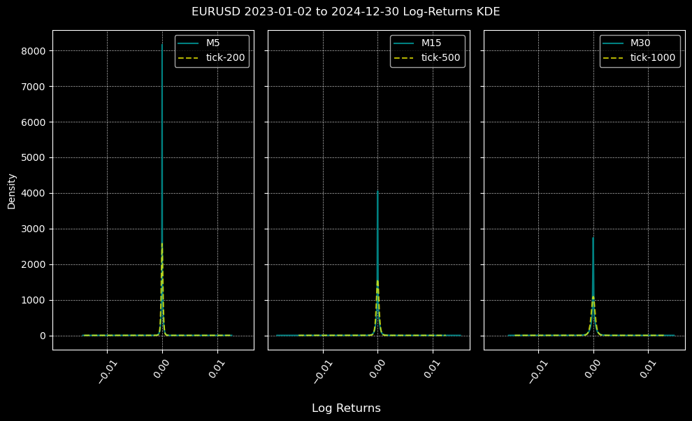
Though none of the log-return distributions are normal, which is to be expected, those created by tick-bars are more normal than those created by time-bars over all timeframes.

Let us perform a more thorough analysis of the statistical properties of time- and tick-bars using the charts below.

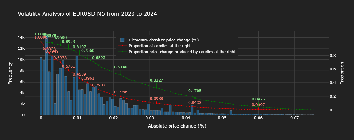
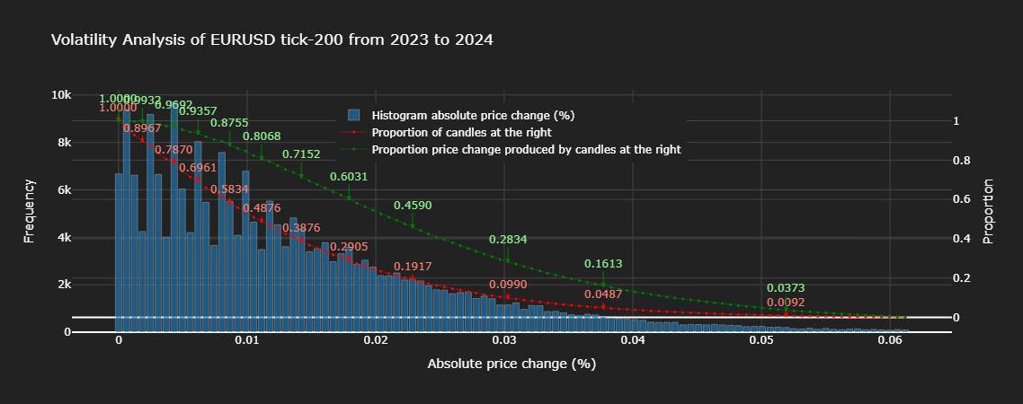
From examining the charts above, we can see that approximately 20% of time-bars explain roughly 51% of the total price change, whereas 20% of tick-bars explain roughly 46% of the total price change. Notably, practically all proportions of tick-bars explain less of the total price change than the same proportion of time-bars, which indicates that tick-bars are better at sampling information than time-bars. A look at the histogram corroborates this, by showing us that the absolute price change of tick-bars follows a much more statistically pleasing distribution (monotonically decreasing) than that of time-bars, which has haphazard variances.

In this, and subsequent articles, our focus will be on applying ML to forex instruments. As these are not traded on a central exchange, volume information is unavailable, and I will therefore limit the scope of this series to time- and tick- bars. The reader should note that I have only described standard bar formations above. For further information on advanced candlestick bars, I recommend this article as it expounds on Marcos López de Prado's work in Advances in Financial Machine Learning, for which seminar notes can be found online.

The Fix: Rewriting Temporal Reality by Creating Bars from Tick Data

Code Implementation

Let us begin by getting data from our terminal, and cleaning it to prevent the possibility of erroneous ticks being used to create our bar data. I will demonstrate how to create time and tick bars. We will be using Python due to the convenience of time-based manipulations in pandas, and its ease of use for ML. 

Step 0: Imports 

These are the imports we will use for the code snippets in this article.

import numpy as np
import pandas as pd
import MetaTrader5 as mt5
import logging
from datetime import datetime as dt

logging.basicConfig(level=logging.INFO, format='%(levelname)s: %(message)s')

Step 1: Data Extraction

def get_ticks(symbol, start_date, end_date):
    """
    Downloads tick data from the MT5 terminal.

    Args:
        symbol (str): Financial instrument (e.g., currency pair or stock).
        start_date, end_date (str or datetime): Time range for data (YYYY-MM-DD).

    Returns:
        pd.DataFrame: Tick data with a datetime index.
    """
    if not mt5.initialize():
        logging.error("MT5 connection not established.")
        raise RuntimeError("MT5 connection error.")

    start_date = pd.Timestamp(start_date, tz='UTC') if isinstance(start_date, str) else (
        start_date if start_date.tzinfo is not None else pd.Timestamp(start_date, tz='UTC')
    )
    end_date = pd.Timestamp(end_date, tz='UTC') if isinstance(end_date, str) else (
        end_date if end_date.tzinfo is not None else pd.Timestamp(end_date, tz='UTC')
    )

    try:
        ticks = mt5.copy_ticks_range(symbol, start_date, end_date, mt5.COPY_TICKS_ALL)
        df = pd.DataFrame(ticks)
        df['time'] = pd.to_datetime(df['time_msc'], unit='ms')
        df.set_index('time', inplace=True)
        df.drop('time_msc', axis=1, inplace=True)
        df = df[df.columns[df.any()]]
        df.info()
    except Exception as e:
        logging.error(f"Error while downloading ticks: {e}")
        return None

    return df

Step 2: Data Cleaning

def clean_tick_data(df: pd.DataFrame,
                    n_digits: int,
                    timezone: str = 'UTC'
                    ) -> Optional[pd.DataFrame]:
    """
    Clean and validate Forex tick data with comprehensive quality checks.

    Args:
        df: DataFrame containing tick data with bid/ask prices and timestamp index
        n_digits: Number of decimal places in instrument price.
        timezone: Timezone to localize/convert timestamps to (default: UTC)

    Returns:
        Cleaned DataFrame or None if empty after cleaning
    """
    if df.empty:
        return None

    df = df.copy(deep=False)  # Work on a copy to avoid modifying the original DataFrame 
    n_initial = df.shape[0] # Store initial row count for reporting

    # 1. Ensure proper datetime index
    # Use errors='coerce' to turn unparseable dates into NaT and then drop them.
    if not isinstance(df.index, pd.DatetimeIndex):
        original_index_name = df.index.name
        df.index = pd.to_datetime(df.index, errors='coerce')
        nan_idx_count = df.index.isnull().sum()
        if nan_idx_count > 0:
            logging.info(f"Dropped {nan_idx_count:,} rows with unparseable timestamps.")
            df = df[~df.index.isnull()]
        if original_index_name:
            df.index.name = original_index_name
    
    if df.empty: # Check if empty after index cleaning
        logging.warning("Warning: DataFrame empty after initial index cleaning")
        return None

    # 2. Timezone handling
    if df.index.tz is None:
        df = df.tz_localize(timezone)
    elif str(df.index.tz) != timezone.upper():
        df = df.tz_convert(timezone)
    
    # 3. Price validity checks
    # Apply rounding and then filtering
    df['bid'] = df['bid'].round(n_digits)
    df['ask'] = df['ask'].round(n_digits)

    # Validate prices
    price_filter = (
        (df['bid'] > 0) &
        (df['ask'] > 0) &
        (df['ask'] > df['bid'])
    )
    
    n_before_price_filter = df.shape[0]
    df = df[price_filter]
    n_filtered_prices = n_before_price_filter - df.shape[0]
    if n_filtered_prices > 0:
        logging.info(f"Filtered {n_filtered_prices:,} ({n_filtered_prices / n_before_price_filter:.2%}) invalid prices.")

    if df.empty: # Check if empty after price cleaning
        logging.warning("Warning: DataFrame empty after price cleaning")
        return None
    
    # Dropping NA values
    initial_rows_before_na = df.shape[0]
    if df.isna().any().any(): # Use .any().any() to check if any NA exists in the whole DF
        na_counts = df.isna().sum()
        na_cols = na_counts[na_counts > 0]
        if not na_cols.empty:
            logging.info(f'Dropped NA values from columns: \n{na_cols}')
            df.dropna(inplace=True)

    n_dropped_na = initial_rows_before_na - df.shape[0]
    if n_dropped_na > 0:
        logging.info(f"Dropped {n_dropped_na:,} ({n_dropped_na / n_before_price_filter:.2%}) rows due to NA values.")

    if df.empty: # Check if empty after NA cleaning
        logging.warning("Warning: DataFrame empty after NA cleaning")
        return None
    
    # 4. Microsecond handling
    if not df.index.microsecond.any():
        logging.warning("Warning: No timestamps with microsecond precision found")
    
    # 5. Duplicate handling
    duplicate_mask = df.index.duplicated(keep='last')
    dup_count = duplicate_mask.sum()
    if dup_count > 0:
        logging.info(f"Removed {dup_count:,} ({dup_count / n_before_price_filter:.2%}) duplicate timestamps.")
        df = df[~duplicate_mask]

    if df.empty: # Check if empty after duplicate cleaning
        logging.warning("Warning: DataFrame empty after duplicate cleaning")
        return None

    # 6. Chronological order
    if not df.index.is_monotonic_increasing:
        logging.info("Sorting DataFrame by index to ensure chronological order.")
        df.sort_index(inplace=True)

    # 7. Final validation and reporting
    if df.empty:
        logging.warning("Warning: DataFrame empty after all cleaning steps.")
        return None
    
    n_final = df.shape[0]
    n_cleaned = n_initial - n_final
    percentage_cleaned = (n_cleaned / n_initial) if n_initial > 0 else 0
    logging.info(f"Cleaned {n_cleaned:,} of {n_initial:,} ({percentage_cleaned:.2%}) datapoints.")

    return df

Step 3: Create Bars and Convert to End-Time

First, we will create some helper functions.

set_resampling_freq

def set_resampling_freq(timeframe: str) -> str:
    """
    Converts an MT5 timeframe to a pandas resampling frequency.

    Args:
        timeframe (str): MT5 timeframe (e.g., 'M1', 'H1', 'D1', 'W1').

    Returns:
        str: Pandas frequency string.
    """
    timeframe = timeframe.upper()
    nums = [x for x in timeframe if x.isnumeric()]
    if not nums:
        raise ValueError("Timeframe must include numeric values (e.g., 'M1').")
    
    x = int(''.join(nums))
    if timeframe == 'W1':
        freq = 'W-FRI'
    elif timeframe == 'D1':
        freq = 'B'
    elif timeframe.startswith('H'):
        freq = f'{x}H'
    elif timeframe.startswith('M'):
        freq = f'{x}min'
    elif timeframe.startswith('S'):
        freq = f'{x}S'
    else:
        raise ValueError("Valid timeframes include W1, D1, Hx, Mx, Sx.")
    
    return freq

calculate_ticks_per_period

def calculate_ticks_per_period(df: pd.DataFrame, timeframe: str = "M1", method: str = 'median', verbose: bool = True) -> int:
    """
    Dynamically calculates the average number of ticks per given timeframe.

    Args:
        df (pd.DataFrame): Tick data.
        timeframe (str): MT5 timeframe.
        method (str): 'median' or 'mean' for the calculation.
        verbose (bool): Whether to print the result.

    Returns:
        int: Rounded average ticks per period.
    """
    freq = set_resampling_freq(timeframe)
    resampled = df.resample(freq).size()
    fn = getattr(np, method)
    num_ticks = fn(resampled.values)
    num_rounded = int(np.round(num_ticks))
    num_digits = len(str(num_rounded)) - 1
    rounded_ticks = int(round(num_rounded, -num_digits))
    rounded_ticks = max(1, rounded_ticks)
    
    if verbose:
        t0 = df.index[0].date()
        t1 = df.index[-1].date()
        logging.info(f"From {t0} to {t1}, {method} ticks per {timeframe}: {num_ticks:,} rounded to {rounded_ticks:,}")
    
    return rounded_ticks

flatten_column_names

def flatten_column_names(df):
    '''
    Joins tuples created by dataframe aggregation 
    with a list of functions into a unified name.
    '''
    return ["_".join(col).strip() for col in df.columns.values]

Now, the main functions used to create bars.

make_bar_type_grouper

def make_bar_type_grouper(
        df: pd.DataFrame,
        bar_type: str = 'tick',
        bar_size: int = 100,
        timeframe: str = 'M1'
) -> tuple[pd.core.groupby.generic.DataFrameGroupBy, int]:
    """
    Create a grouped object for aggregating tick data into time/tick/dollar/volume bars.

    Args:
        df: DataFrame with tick data (index should be datetime for time bars).
        bar_type: Type of bar ('time', 'tick', 'dollar', 'volume').
        bar_size: Number of ticks/dollars/volume per bar (ignored for time bars).
        timeframe: Timeframe for resampling (e.g., 'H1', 'D1', 'W1').

    Returns:
        - GroupBy object for aggregation
        - Calculated bar_size (for tick/dollar/volume bars)
    """
    # Create working copy (shallow is sufficient)
    df = df.copy(deep=False)  # OPTIMIZATION: Shallow copy here only once
    
    # Ensure DatetimeIndex
    if not isinstance(df.index, pd.DatetimeIndex):
        try:
            df = df.set_index('time')
        except KeyError:
            raise TypeError("Could not set 'time' as index")

    # Sort if needed
    if not df.index.is_monotonic_increasing:
        df = df.sort_index()

    # Time bars
    if bar_type == 'time':
        freq = set_resampling_freq(timeframe)
        bar_group = (df.resample(freq, closed='left', label='right') # includes data upto, but not including, the end of the period
                    if not freq.startswith(('B', 'W')) 
                    else df.resample(freq))
        return bar_group, 0  # bar_size not used

    # Dynamic bar sizing
    if bar_size == 0:
        if bar_type == 'tick':
            bar_size = calculate_ticks_per_period(df, timeframe)
        else:
            raise NotImplementedError(f"{bar_type} bars require non-zero bar_size")

    # Non-time bars
    df['time'] = df.index  # Add without copying
    
    if bar_type == 'tick':
        bar_id = np.arange(len(df)) // bar_size
    elif bar_type in ('volume', 'dollar'):
        if 'volume' not in df.columns:
            raise KeyError(f"'volume' column required for {bar_type} bars")
        
        # Optimized cumulative sum
        cum_metric = (df['volume'] * df['bid'] if bar_type == 'dollar' 
                      else df['volume'])
        cumsum = cum_metric.cumsum()
        bar_id = (cumsum // bar_size).astype(int)
    else:
        raise NotImplementedError(f"{bar_type} bars not implemented")

    return df.groupby(bar_id), bar_size

make_bars

def make_bars(tick_df: pd.DataFrame,
              bar_type: str = 'tick',
              bar_size: int = 0,
              timeframe: str = 'M1',
              price: str = 'midprice',
              verbose=True):
    '''
    Create OHLC data by sampling ticks using timeframe or a threshold.

    Parameters
    ----------
    tick_df: pd.DataFrame
        tick data
    bar_type: str
        type of bars to create from ['tick', 'time', 'volume', 'dollar']
    bar_size: int 
        default 0. bar_size when bar_type != 'time'
    timeframe: str
        MT5 timeframe (e.g., 'M5', 'H1', 'D1', 'W1').
        Used for time bars, or for tick bars if bar_size = 0.
    price: str
        default midprice. If 'bid_ask', columns (bid_open, ..., bid_close), 
        (ask_open, ..., ask_close) are included.
    verbose: bool
        print information about the data

    Returns
    -------
    pd.DataFrame with columns [open, high, low, close, median_price, tick_volume, volume]
    '''    
    if 'midprice' not in tick_df:
        tick_df['midprice'] = (tick_df['bid'] + tick_df['ask']) / 2

    bar_group, bar_size_ = make_bar_type_grouper(tick_df, bar_type, bar_size, timeframe)
    ohlc_df = bar_group['midprice'].ohlc().astype('float64')
    ohlc_df['tick_volume'] = bar_group['bid'].count() if bar_type != 'tick' else bar_size_
    
    if price == 'bid_ask':
        # Aggregate OHLC data for every bar_size rows
        bid_ask_df = bar_group.agg({k: 'ohlc' for k in ('bid', 'ask')})
        # Flatten MultiIndex columns
        col_names = flatten_column_names(bid_ask_df)
        bid_ask_df.columns = col_names
        ohlc_df = ohlc_df.join(bid_ask_df)

    if 'volume' in tick_df:
        ohlc_df['volume'] = bar_group['volume'].sum()

    if bar_type == 'time':
        ohlc_df.ffill(inplace=True)
    else:
        end_time =  bar_group['time'].last()
        ohlc_df.index = end_time + pd.Timedelta(microseconds=1) # ensure end time is after event
	df.drop('time', axis=1, inplace=True) # Remove 'time' column


        # drop last bar due to insufficient ticks
        if len(tick_df) % bar_size_ > 0: 
            ohlc_df = ohlc_df.iloc[:-1]

    if verbose:
        if bar_type != 'time':
            tm = f'{bar_size_:,}'
            if bar_type == 'tick' and bar_size == 0:
                tm = f'{timeframe} - {bar_size_:,} ticks'
            timeframe = tm
        print(f'\nTick data - {tick_df.shape[0]:,} rows')
        print(f'{bar_type}_bar {timeframe}')
        ohlc_df.info()
    
    # Remove timezone info from DatetimeIndex
    try:
	ohlc_df = ohlc_df.tz_convert(None)
    except:
	pass
    
    return ohlc_df

The volatility analysis plots we used above were created using the following code:

import plotly.graph_objects as go
import numpy as np
import pandas as pd

def plot_volatility_analysis_of_bars(df, symbol, start, end, freq, thres=.01, bins=100):
    """
    Plot the volatility analysis of bars using Plotly.
    df: DataFrame containing the data with 'open' and 'close' columns.
    symbol: Symbol of the asset.    
    start: Start date of the data.
    end: End date of the data.
    freq: Frequency of the data.
    thres: Threshold for filtering large values, e.g., 1-.01 for 99th quantile.
    bins: Number of bins for the histogram.
    """
    abs_price_changes = (df['close'] / df['open'] - 1).mul(100).abs()
    thres = abs_price_changes.quantile(1 - thres)
    abs_price_changes = abs_price_changes[abs_price_changes < thres] # filter out large values for visualization

    # Calculate Histogram
    counts, bins = np.histogram(abs_price_changes, bins=bins)
    bins = bins[:-1] # remove the last bin edge

    # Calculate Proportions
    total_counts = len(abs_price_changes)
    proportion_candles_right = []
    proportion_price_change_right = []

    for i in range(len(bins)):
        candles_right = abs_price_changes[abs_price_changes >= bins[i]]
        count_right = len(candles_right)
        proportion_candles_right.append(count_right / total_counts)
        proportion_price_change_right.append(np.sum(candles_right) / np.sum(abs_price_changes))

    fig = go.Figure()

    # Histogram with Hover Template
    fig.add_trace(
        go.Bar(x=bins, y=counts, 
               name='Histogram absolute price change (%)',
               marker=dict(color='#1f77b4'), 
               hovertemplate='<b>Bin: %{x:.2f}</b><br>Frequency: %{y}',  # Custom hover text
               yaxis='y1',
               opacity=.65))

    ms = 3 # marker size
    lw = .5 # line width
    
    # Proportion of Candles at the Right with Hover Text
    fig.add_trace(
        go.Scatter(x=bins, y=proportion_candles_right, 
                   name='Proportion of candles at the right',
                   mode='lines+markers', 
                   marker=dict(color='red', size=ms), 
                   line=dict(width=lw),
                   hovertext=[f"Bin: {x:.2f}, Proportion: {y:.4f}" 
                              for x, y in zip(bins, proportion_candles_right)],  # Hover text list
                   hoverinfo='text',  # Show only the 'text' from hovertext
                   yaxis='y2'))
    

    # Proportion Price Change Produced by Candles at the Right with Hover Text
    fig.add_trace(
        go.Scatter(x=bins, y=proportion_price_change_right, 
                   name='Proportion price change produced by candles at the right',
                   mode='lines+markers', 
                   marker=dict(color='green', size=ms), 
                   line=dict(width=lw),
                   hovertext=[f"Bin: {x:.2f}, Proportion: {y:.4f}" 
                              for x, y in zip(bins, proportion_price_change_right)], # Hover text list
                   hoverinfo='text',  # Show only the 'text' from hovertext
                   yaxis='y2'))
    
    # Indices of proportion_price_change_right at 10% intervals
    search_idx = [.01, .05] + np.linspace(.1, 1., 10).tolist()
    price_idxs = np.searchsorted(sorted(proportion_candles_right), search_idx, side='right')
    for ix in price_idxs:  # Add annotations for every step-th data point as an example
        x = bins[-ix]
        y = proportion_candles_right[-ix]
        fig.add_annotation(
            x=x,
            y=y,
            text=f"{y:.4f}",  # Display the proportion value with 4 decimal points
            showarrow=True,
            arrowhead=1,
            ax=0,
            ay=-15,  # Offset for the annotation text
            font=dict(color="salmon"),
            arrowcolor="red",
            yref='y2'
        )

        y = proportion_price_change_right[-ix]
        fig.add_annotation(
            x=x,
            y=y,
            text=f"{y:.4f}",  # Display the proportion value with 4 decimal points
            showarrow=True,
            arrowhead=1,
            ax=0,
            ay=-25,  # Offset for the annotation text
            font=dict(color="lightgreen"),
            arrowcolor="green",
            yref='y2'
        )

    # Layout Configuration with Legend Inside
    fig.update_layout(
        title=f'Volatility Analysis of {symbol} {freq} from {start} to {end}',
        xaxis_title='Absolute price change (%)',
        yaxis_title='Frequency',
        yaxis2=dict(
            title='Proportion',
            overlaying='y',
            side='right',
            gridcolor='#444'  # Set grid color for the secondary y-axis
        ),
        plot_bgcolor='#222',  # Dark gray background
        paper_bgcolor='#222',
        font=dict(color='white'),
        xaxis=dict(gridcolor='#444'),  # Set grid color for the primary x-axis
        yaxis=dict(gridcolor='#444'),   # Set grid color for the primary y-axis
        legend=dict(
            x=0.3,  # Adjust x coordinate (0 to 1)
            y=0.95,  # Adjust y coordinate (0 to 1)
            traceorder="normal",  # Optional: maintain trace order
            font=dict(color="white")  # Optional: set legend text color
        ),
        # width=750,  # Set width of the figure
        # height=480,  # Set height of the figure
    )

    return fig

Now that we have seen how to create structured data from our tick data in the form of time- or tick-bars, let's see if some of the claims we made about the statistical properties of tick-bars being superior to those of time-bars hold. We will use EURUSD 2023 tick data, which is attached in the files below.

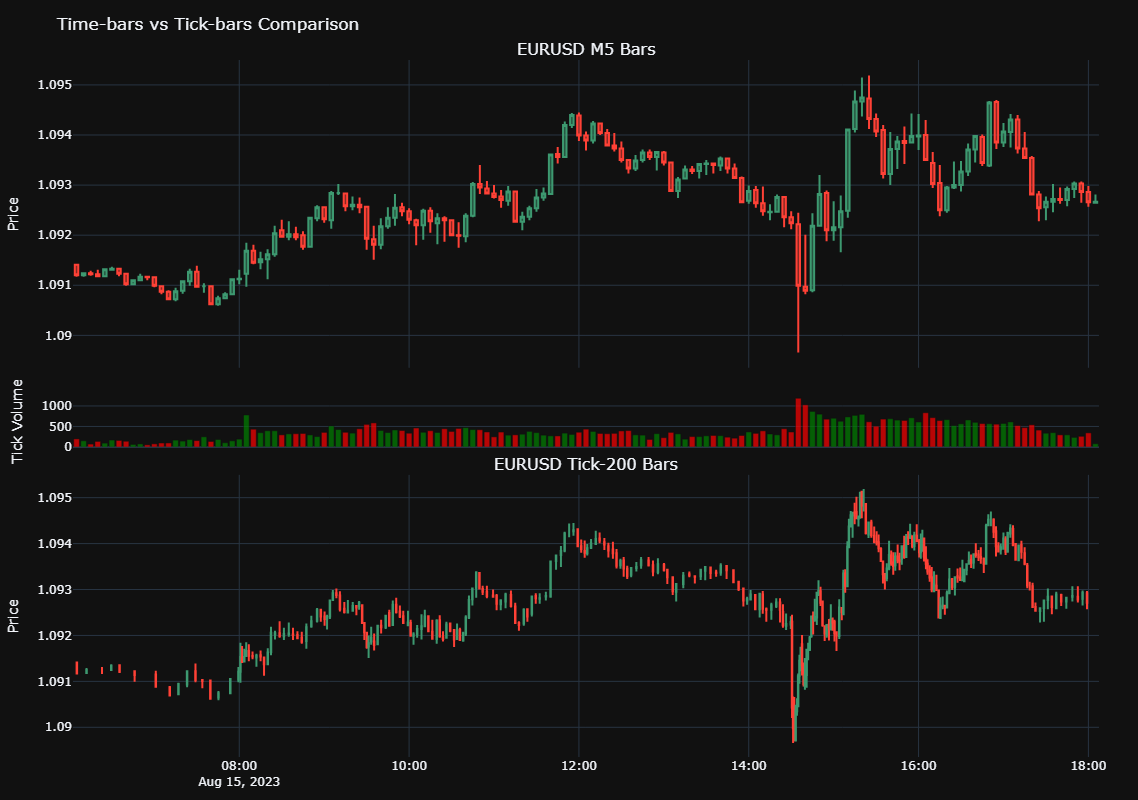
If you look closely at the areas where there is high tick-volume in the M5 chart, such as between 14:00 and 16:00, you will notice that the bars formed in the Tick-200 chart overlap due to the increased sampling in this high-activity period. Conversely, the tick-bars between 06:00 and 08:00 are sparse and have large gaps between them. This illustrates why tick-bars are referred to as activity-driven bars, in contrast to time-bars which uniformly sample data over a fixed time horizon.

Scalability and Hardware Recommendations

Working with high-frequency tick data and constructing specialized bars can be computationally intensive, especially with large historical datasets. For optimal performance and efficient processing, we recommend the following computing setup:

• RAM: A minimum of 16GB RAM is advisable, with 32GB or more preferred for extensive backtesting or processing years of tick data.
• CPU: A multi-core CPU (e.g., Intel i7/i9 or AMD Ryzen 7/9) is highly recommended. The ability to parallelize data processing tasks across multiple cores will significantly reduce computation time.
• Parallelization Strategies: Consider implementing parallel processing techniques in your Python code. Libraries such as Dask for distributed computing or Python's built-in multiprocessing module can be invaluable for speeding up data preparation, feature engineering, and backtesting simulations on large datasets.

Next Steps

To effectively apply the concepts discussed in this article and prepare for the subsequent parts of this series, we recommend the following actionable steps:

1. Implement Timestamp Correction: Integrate the provided code snippets into your data ingestion pipeline to ensure all MetaTrader 5 data is correctly timestamped and free from look-ahead bias.
2. Experiment with Bar Types: Beyond tick bars, explore other specialized bar types such as volume bars or dollar bars. Observe how these different sampling methods impact the characteristics of your dataset and their potential benefits for your specific trading strategies.
3. Prepare Your Dataset: With clean, unbiased data now in hand, begin organizing and preparing your dataset for the next stages of the machine learning pipeline. In Part 2, we will delve into advanced feature engineering and labelling techniques.

Coming up next in our series, we'll dive into one of the most pivotal steps in building powerful supervised machine learning models for finance—label creation. While traditional fixed-time horizon methods dominate much of the literature, they often fall short in capturing the true dynamics of financial markets.

That's why in the next article, we'll explore two of Dr. Marcos López de Prado's groundbreaking alternatives: the triple-barrier method and trend-scanning method. These techniques don't just rethink labeling—they redefine it.

If you've ever questioned whether your labels are truly aligned with how markets behave, this is the insight you've been waiting for.

Conclusion

In this foundational article, we have meticulously addressed and provided solutions for the critical "MetaTrader 5 timestamp trap." We demonstrated how improper timestamp handling can introduce severe data leakage, leading to flawed models and unreliable trading signals. By implementing robust timestamp correction mechanisms and leveraging the power of tick-bar construction, we have successfully laid the groundwork for building high-integrity datasets. This fundamental fix is paramount for ensuring the validity of your research, the accuracy of your backtests, and ultimately, the reliability of your machine learning models in algorithmic trading. This crucial first step is essential for any serious quantitative practitioner aiming to develop truly effective and trustworthy trading systems.

In the attached documents you will find the code used above, as well as some utility functions for logging into the MetaTrader 5 terminal using the Python API.