Foundation Models for Trading (Part II): Decoding, Autoregression, and an Exact KV-Cache

Introduction

In Part 1 we built and verified the front half of a native MQL5 port of Kronos: the weight bridge from PyTorch, the preprocessing, the Binary Spherical Quantization that turns a candle into a pair of hierarchical tokens, and the transformer block assembled from primitive matrix operations. The encoder reproduced the reference tokens exactly. We stopped at the point where a window of candles has become a sequence of tokens.

This part moves to the other half of the model. We build the decoder that turns tokens back into candles, the predictor that generates new tokens one step at a time, and the autoregressive loop that ties them together into a multi-bar forecast. Along the way we meet the subtle traps that cost real debugging time: a cross-attention head that uses a different number of heads than the rest of the model, a rotary embedding that rotates every key at the same position, and an embedding that is scaled in one place but left raw in another. Each is the kind of mistake that runs without error and quietly corrupts the output.

Then we make it fast. A first working port generated a forecast slowly enough to be impractical for any real study. Two fixes together cut the per-step time by roughly four and a half times: a key/value cache that skips the work the loop was repeating, and a weight-transpose fix that the profiler surfaced in a place intuition would not have looked. By the end of this part, the full pipeline runs end to end, verified stage by stage against the PyTorch reference: a window of candles goes in, and a multi-bar forecast in real price units comes out.

We will cover:

1. From Tokens Back to Candles: The Decoder
2. The Predictor's Hierarchical Embedding
3. Loading the Predictor's Weights
4. decode_s1: Predicting the Coarse Token
5. decode_s2 and the Cross-Attention Traps
6. Sampling the Next Token
7. The Autoregressive Loop
8. A KV-Cache That Stays Exact
9. Making It Fast: Profiling and Pre-Transposed Weights
10. Conclusion

From Tokens Back to Candles: The Decoder

The decoder is the mirror of the encoder from Part 1, and it reuses the same transformer machinery. Where the encoder went from six features to a 20-bit code, the decoder goes from the code back to six features. Given the two token ids for each bar, it rebuilds the bipolar BSQ code, projects it up to model width, runs a stack of causal blocks, and projects down to the normalized OHLCVA bar.

//+---------------------------------------------------------------+
//| Decode hierarchical token ids into a normalized OHLCVA window.|
//|   s1_ids,s2_ids : input token ids, length L                   |
//|   recon_norm    : output (L, 6), still z-scored (denormalize  |
//|                   separately with the window's mean/std)      |
//+---------------------------------------------------------------+
bool              Decode(const int &s1_ids[], const int &s2_ids[], matrix &recon_norm)
  {
   int L = ArraySize(s1_ids);
   if(L == 0 || ArraySize(s2_ids) != L)
     { PrintFormat("CKronosDecoder::Decode: bad id lengths (%d / %d)", L, ArraySize(s2_ids)); return false; }

//--- indices_to_bits (half): each row is the 20-dim bipolar code (LSB-first)
   matrix code = matrix::Zeros((ulong)L, KR_CODEBOOK_DIM);
   double row[];
   for(int t = 0; t < L; t++)
     {
      KronosBSQ_IndicesToCode(s1_ids[t], s2_ids[t], row);   // verified BSQ math
      for(int k = 0; k < KR_CODEBOOK_DIM; k++)
         code[t][k] = row[k];
     }
//--- post_quant_embed: 20 -> d_model
   matrix z = LinearT(code, m_pqW);
   AddRowBias(z, m_pqB);
//--- (n_dec_layers - 1) causal pre-norm blocks
   for(int b = 0; b < m_blocks; b++)
      z = TransformerBlock(z, m_n1[b],
                           m_Wq[b], m_bq[b], m_Wk[b], m_bk[b],
                           m_Wv[b], m_bv[b], m_Wo[b], m_bo[b],
                           m_heads, m_n2[b], m_W1[b], m_W3[b], m_W2[b]);
//--- head: d_model -> 6 (normalized OHLCVA)
   recon_norm = LinearT(z, m_headW);
   AddRowBias(recon_norm, m_headB);
   return true;
  }

The KronosBSQ_IndicesToCode call is the same verified BSQ math from Part 1, run in reverse: each bit becomes a bipolar value on the hypersphere. After that, the structure is identical to the encoder, embed, blocks, project, with two differences. The projection in is post_quant_embed (20 to model width) instead of embed (6 to model width), and the projection out is the head (model width to 6) that produces the reconstructed bar. The same n - 1 block-count quirk from the tokenizer applies here, so a configured four decoder layers gives three blocks.

The output is still in normalized space. To get prices, the caller denormalizes with the mean and standard deviation of the original context window, exactly the statistics saved during preprocessing.

Verification continues on the same ladder Part 1 built, but with one change. The encoder's target was discrete token ids, checked for exact integer equality. Everything in this part, the decoder's reconstruction, the s1 logits, the s2 logits, is continuous, so the harnesses swap the exact-equality test for a maximum-absolute-error test against a small tolerance. KronosVerifyDecoder is representative; it loads the golden recon_norm, runs the MQL5 decoder on the same tokens, and scans for the worst cell:

//--- float comparison: max-abs and mean-abs error, plus worst cell
double maxerr = 0.0, sumerr = 0.0;
int wr = -1, wc = -1;
for(int i = 0; i < L; i++)
   for(int j = 0; j < KR_NFEAT; j++)
     {
      double e = MathAbs(mine[i][j] - ref[i][j]);
      sumerr += e;
      if(e > maxerr)
        {
         maxerr = e;
         wr = i;
         wc = j;
        }
     }
double meanerr = sumerr / (double)(L * KR_NFEAT);

The pass condition is simply maxerr <= tol, and the harness prints the worst cell so a real mismatch can be localized rather than just flagged. For the decoder, the maximum absolute error is about 1.8e-06, the expected size of difference between MQL5 double and the reference float32. The predictor harnesses (KronosVerifyPredictorS1 and KronosVerifyPredictorS2) apply the same test to the logits, and additionally confirm the argmax matches, so the token the model would actually pick is reproduced. The maximum errors come out at about 4.7e-06 and 9.8e-06 respectively, as we reach each stage below.

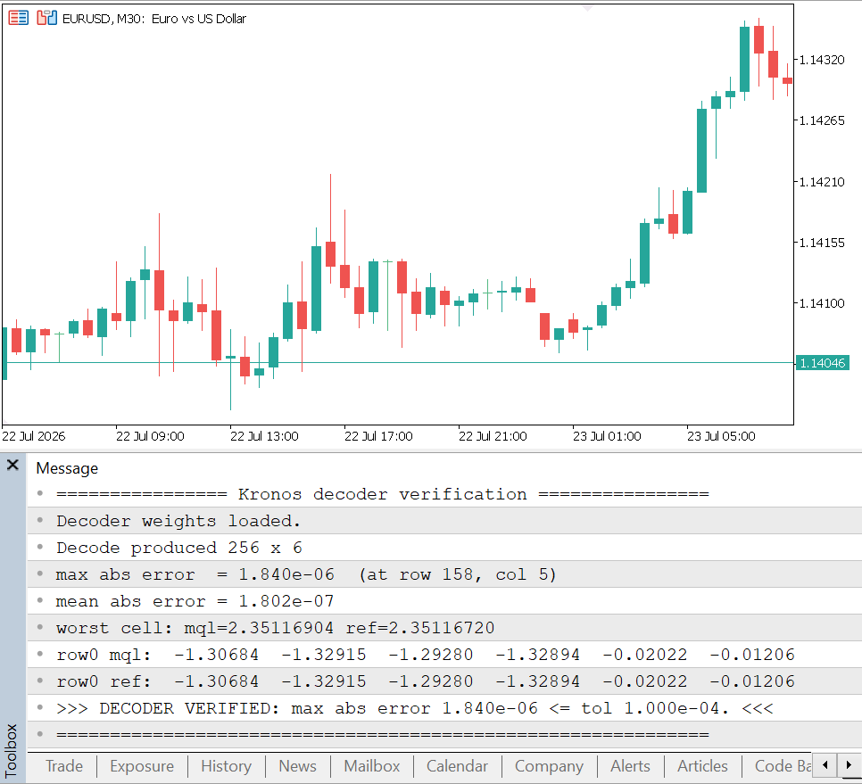
Fig. 1. The decoder verification harness reporting a maximum absolute error around 1.8e-06 against the reference reconstruction

The Predictor's Hierarchical Embedding

The predictor is a separate, larger transformer, 512-dimensional and eight layers, that operates on the token sequence and predicts the next token. Before any block runs, each token has to become a vector the transformer can process, and Kronos builds that input from three ingredients: the two subtoken embeddings, fused, plus a temporal embedding from the bar's time stamp.

The EmbedRows method assembles it. Each subtoken id indexes its own learned embedding table, emb_s1 and emb_s2, and the looked-up rows are scaled by the square root of the model width before being concatenated and passed through the fusion_proj linear layer. Then the five temporal tables, minute, hour, weekday, day, and month, are added in.

//+---------------------------------------------------------------+
//| Build the transformer input rows for the given tokens/stamp:  |
//| HierarchicalEmbedding( fusion_proj(cat(emb_s1*sqrt d,         |
//| emb_s2*sqrt d)) ) + TemporalEmbedding(stamp). Shared by the   |
//| full DecodeS1 and the cached prime/step paths so they embed   |
//| identically. out is (L, d_model).                             |
//+---------------------------------------------------------------+
void              EmbedRows(const int &s1_ids[], const int &s2_ids[], const matrix &stamp, matrix &out)
  {
   int L = ArraySize(s1_ids);
   double scale = MathSqrt((double)m_dm);

   matrix e1, e2;
   EmbedTokens(s1_ids, m_embS1, scale, e1);
   EmbedTokens(s2_ids, m_embS2, scale, e2);

   matrix cat = matrix::Zeros((ulong)L, 2 * m_dm);
   for(int t = 0; t < L; t++)
     {
      for(ulong j = 0; j < m_dm; j++)
         cat[t][j]        = e1[t][j];
      for(ulong j = 0; j < m_dm; j++)
         cat[t][m_dm + j] = e2[t][j];
     }
   out = LinearT(cat, m_fusionW);
   AddRowBias(out, m_fusionB);

   if(stamp.Rows() == (ulong)L && stamp.Cols() >= 5)
     {
      AddTimeEmbed(stamp, 0, m_teMin,  out);
      AddTimeEmbed(stamp, 1, m_teHour, out);
      AddTimeEmbed(stamp, 2, m_teWday, out);
      AddTimeEmbed(stamp, 3, m_teDay,  out);
      AddTimeEmbed(stamp, 4, m_teMon,  out);
     }
  }

EmbedRows is the assembler; the two lookups it calls are one level down. EmbedTokens is where the scaling actually happens, each id indexes its table row and the row is multiplied by scale:

//+---------------------------------------------------------------+
//| Embedding lookup with scaling: row `id` of the table times    |
//| the given scale (sqrt(d_model) for the hierarchical embed).   |
//+---------------------------------------------------------------+
void              EmbedTokens(const int &ids[], const matrix &table, double scale, matrix &out)
  {
   int L = ArraySize(ids);
   out = matrix::Zeros((ulong)L, m_dm);
   for(int t = 0; t < L; t++)
     {
      ulong id = (ulong)ids[t];
      for(ulong j = 0; j < m_dm; j++)
         out[t][j] = table[id][j] * scale;
     }
  }

Passing scale = sqrt(d_model) here is what makes this the hierarchical embedding. The same table, looked up without that scale, reappears in the next section as the sibling embedding, and confusing the two is trap one of decode_s2. AddTimeEmbed is the temporal half, adding one table's row per bar:

//+---------------------------------------------------------------+
//| Add one temporal table's contribution: for each row t, add    |
//| table row stamp[t][col] to x.                                 |
//+---------------------------------------------------------------+
void              AddTimeEmbed(const matrix &stamp, int col, const matrix &table, matrix &x)
  {
   ulong L = x.Rows();
   for(ulong t = 0; t < L; t++)
     {
      ulong idx = (ulong)MathRound(stamp[t][col]);   // stamp stored as float
      for(ulong j = 0; j < m_dm; j++)
         x[t][j] += table[idx][j];
     }
  }

The stamp is stored as a float matrix, so each index is rounded back to an integer before it indexes the table, the MathRound above. This is also the concrete place the Part 1 weekday remap earns its keep: the table has exactly one row per valid value, so a weekday index of 7, which the un-remapped MQL5 convention would produce, indexes past the end of a seven-row table. The remap is what keeps idx in range. The five temporal contributions, minute through month, are simply summed onto the fused token embedding.

Fig. 2. Building one transformer input row: the s1 and s2 embeddings are scaled and fused, then the five temporal embeddings for the bar's time stamp are added

Loading the Predictor's Weights

Before any of that machinery runs, the weights have to be loaded into the class members it reads. This is where the pre-transpose decision from Part 1 becomes concrete, because the loader chosen for each tensor depends on how the tensor is used. Two rules cover everything. A tensor used as a LinearT weight is stored transposed with KronosLoadMatrixT, so the forward pass is a plain matrix multiply. A tensor used as a lookup table, indexed by a token id or a stamp value, is kept row-major with plain KronosLoadMatrix, because we index its rows directly and never multiply by it. The predictor's embedding and head load shows both rules side by side:

bool ok = true;
//--- embeddings
//--- emb_s1/emb_s2 are lookup tables (indexed by token id) -> keep row-major
ok &= KronosLoadMatrix(F("embedding_emb_s1_weight"),    KR_PRED_VOCAB, m_dm, m_embS1);
ok &= KronosLoadMatrix(F("embedding_emb_s2_weight"),    KR_PRED_VOCAB, m_dm, m_embS2);
//--- fusion_proj is a LinearT weight -> store transposed
ok &= KronosLoadMatrixT(F("embedding_fusion_proj_weight"), m_dm, 2 * m_dm, m_fusionW);
ok &= KronosLoadVector(F("embedding_fusion_proj_bias"), m_dm,               m_fusionB);
ok &= KronosLoadMatrix(F("time_emb_minute_embed_weight"),  60, m_dm, m_teMin);
ok &= KronosLoadMatrix(F("time_emb_hour_embed_weight"),    24, m_dm, m_teHour);
ok &= KronosLoadMatrix(F("time_emb_weekday_embed_weight"),  7, m_dm, m_teWday);
ok &= KronosLoadMatrix(F("time_emb_day_embed_weight"),     32, m_dm, m_teDay);
ok &= KronosLoadMatrix(F("time_emb_month_embed_weight"),   13, m_dm, m_teMon);
//--- final norm + s1 head
ok &= KronosLoadVector(F("norm_weight"),          m_dm,                m_normW);
ok &= KronosLoadMatrixT(F("head_proj_s1_weight"), KR_PRED_VOCAB, m_dm, m_projS1W);
ok &= KronosLoadVector(F("head_proj_s1_bias"),    KR_PRED_VOCAB,       m_projS1B);

The temporal table sizes are worth reading off directly: 60 minutes, 24 hours, 7 weekdays, 32 days, 13 months. The seven-row weekday table is exactly why the Part 1 remap is not optional, an un-remapped index of 7 would read past the end of that table. The generous day and month sizes (32 and 13 rather than 31 and 12) simply leave room for one-based indexing without special-casing. The string passed to F is the manifest name from the export in Part 1, with every non-alphanumeric character mapped to an underscore, so embedding.fusion_proj.weight in PyTorch became embedding_fusion_proj_weight.bin on disk and is requested here by that exact name. The eight transformer blocks are loaded the same way in a loop, with the block index formatted into the name (transformer_0_, transformer_1_, and so on) to match the ModuleList keys. This is the join between the offline export and the running engine: the manifest is the contract, and these loaders read against it.

decode_s1: Predicting the Coarse Token

With the input rows built, predicting the coarse token is a standard decoder-only forward pass. The token rows go through eight causal transformer blocks, a final RMSNorm produces what the model calls the context, and a linear head projects the context to a 1024-way logit vector over the s1 vocabulary.

//+---------------------------------------------------------------+
//| decode_s1: returns s1_logits (L, 1024) and context            |
//| (L, d_model). stamp is (L, 5) float with columns              |
//| [minute,hour,weekday,day,month], weekday already in the       |
//| pandas convention (Mon=0..Sun=6).                             |
//+---------------------------------------------------------------+
bool              DecodeS1(const int &s1_ids[], const int &s2_ids[], const matrix &stamp,
              matrix &s1_logits, matrix &context)
  {
   int L = ArraySize(s1_ids);
   if(L == 0 || ArraySize(s2_ids) != L)
     { PrintFormat("DecodeS1: bad id lengths (%d / %d)", L, ArraySize(s2_ids)); return false; }

   matrix x;
   EmbedRows(s1_ids, s2_ids, stamp, x);   // HierarchicalEmbedding + TemporalEmbedding
//--- 8 causal pre-norm transformer blocks
   for(int b = 0; b < m_blocks; b++)
      x = TransformerBlock(x, m_n1[b],
                           m_Wq[b], m_bq[b], m_Wk[b], m_bk[b],
                           m_Wv[b], m_bv[b], m_Wo[b], m_bo[b],
                           m_heads, m_n2[b], m_W1[b], m_W3[b], m_W2[b]);
//--- final RMSNorm -> this is "context" returned for decode_s2
   context = RMSNorm(x, m_normW);
//--- s1 head: d_model -> 1024
   s1_logits = LinearT(context, m_projS1W);
   AddRowBias(s1_logits, m_projS1B);
   return true;
  }

There is one quiet but important difference from the tokenizer here, and it is a trap precisely because the code looks so similar. The loop runs over m_blocks, and for the predictor m_blocks is set to the full layer count, eight, not the n - 1 that the tokenizer used. The tokenizer's block list is built with range(n_layers - 1); the predictor's is built with range(n_layers). If you copy the tokenizer's quirk into the predictor by reflex, you silently drop a block and the logits are wrong. The two must be configured differently.

Port trap: the tokenizer uses n - 1 blocks; the predictor uses the full n. Same-looking loop, different count. The predictor's eight blocks are all present.

The context this method returns is not just an intermediate, it is reused directly by the next stage. It is the post-final-norm representation of every position, and decode_s2's cross-attention will read across all of it. The s1 logits are verified against the reference at about 4.7e-06, with the argmax matching, so the coarse token the model would pick is reproduced exactly.

decode_s2 and the Cross-Attention Traps

Predicting the fine token is where the port earns its scars. The fine token is not predicted from the context alone; it is conditioned on the coarse token just chosen, through a small cross-attention layer Kronos calls the dependency-aware layer. This single method packs three separate traps, and each one produced output that looked almost right, which is the dangerous kind of wrong.

//+---------------------------------------------------------------+
//| decode_s2: context (L, d_model) from decode_s1 plus the chosen|
//| s1 ids. Returns s2_logits (L, 1024).                          |
//|                                                               |
//| s1_ids may have length L (one sibling per position) or length |
//| 1 (a single sibling broadcast across all L context rows). The |
//| length-1 case mirrors the reference capture (s1_pick = argmax |
//| of the last step), where PyTorch broadcasts (L,d)+(1,d) and   |
//| the single query sits at RoPE position 0.                     |
//+---------------------------------------------------------------+
bool              DecodeS2(const matrix &context, const int &s1_ids[], matrix &s2_logits)
  {
   ulong L = context.Rows();
   int   Q = ArraySize(s1_ids);
   if(L == 0 || (Q != (int)L && Q != 1))
     { PrintFormat("DecodeS2: length mismatch (ids %d, ctx %I64u)", Q, L); return false; }

//--- sibling_embed = raw emb_s1 table rows (NO sqrt(d) scale here).
//--- Q rows: either L (per-position) or 1 (broadcast).
   matrix sib = matrix::Zeros((ulong)Q, m_dm);
   for(int t = 0; t < Q; t++)
     {
      ulong id = (ulong)s1_ids[t];
      for(ulong j = 0; j < m_dm; j++)
         sib[t][j] = m_embS1[id][j];
     }
//--- cross-attention: q = sibling_embed (Q rows), k/v = context (L rows),
//--- n_heads=4, non-causal. attn has Q rows.
   matrix attn = CrossMHA(sib, context,
                          m_cWq, m_cBq, m_cWk, m_cBk,
                          m_cWv, m_cBv, m_cWo, m_cBo,
                          KR_DEP_N_HEADS);
//--- dep_layer: RMSNorm(context + attn). Broadcast attn row 0 across
//--- all L context rows when Q == 1 (matches PyTorch (L,d)+(1,d)).
   matrix sum = matrix::Zeros(L, m_dm);
   for(ulong i = 0; i < L; i++)
     {
      ulong ar = (Q == 1) ? 0 : i;
      for(ulong j = 0; j < m_dm; j++)
         sum[i][j] = context[i][j] + attn[ar][j];
     }
   matrix x2 = RMSNorm(sum, m_depNormW);
//--- s2 head: d_model -> 1024
   s2_logits = LinearT(x2, m_projS2W);
   AddRowBias(s2_logits, m_projS2B);
   return true;
  }

Trap one: the sibling embedding is raw. The query of this cross-attention is the embedding of the chosen s1 token, and it uses the same emb_s1 table we used in the hierarchical embedding, but without the square-root-of-d scaling. In the source, the hierarchical embedding multiplies by that factor inside its own forward, while here the table is indexed directly. Apply the scaling out of habit and every query is the wrong magnitude.

Trap two: this cross-attention uses four heads, not eight. The rest of the predictor uses eight attention heads. The dependency-aware layer is constructed without specifying a head count, so it falls back to a default of four, which makes its head dimension 128 instead of 64. That difference changes how the columns are split into heads and, critically, the length of the rotary frequency table. Use eight here and the rotary embedding is silently corrupted. This is why the call passes KR_DEP_N_HEADS, defined as 4, rather than the predictor's head count.

Trap three: the rotary cache is sized to the query, then applied to the keys. This is the most subtle of the three, and it lives inside CrossMHA. The rotary embedding builds its cosine and sine cache from the query length and applies that same cache to the keys. At inference the query is a single broadcast s1 pick, so its length is one, which means every key gets rotated at position zero rather than at its own position. Rotating keys by their true positions is the natural thing to write, and it is wrong: it gave a maximum error of 0.57 while the final argmax still happened to match, a partial failure that is easy to miss. The fix is to reuse the query-length table for the keys, indexing each key by its position only when the query and key lengths are equal.

All three traps are visible in the cross-attention function itself. It is worth reading in full, because unlike the causal MHA from Part 1, every line here that differs from ordinary self-attention encodes one of the three:

//+------------------------------------------------------------------+
//| Non-causal multi-head CROSS-attention with RoPE (inference).     |
//| q from Xq (sibling embed), k/v from Xkv (context); each query    |
//| attends to ALL key positions. q/k/v/out carry a bias. The        |
//| predictor's dep_layer uses n_heads=4 (head_dim=128), NOT 8.      |
//|                                                                  |
//| RoPE quirk (matches RotaryPositionalEmbedding.forward): the      |
//| cos/sin cache is sized to the QUERY length and the same cache is |
//| applied to the keys. So when Tq==1 (a single broadcast s1 pick)  |
//| every key is rotated at position 0; when Tq==Tk keys rotate by   |
//| their own positions. We index the key rotation by (Tq==1 ? 0:j), |
//| reusing the query's table.                                       |
//+------------------------------------------------------------------+
matrix CrossMHA(const matrix &Xq, const matrix &Xkv,
                const matrix &Wq, const vector &bq,
                const matrix &Wk, const vector &bk,
                const matrix &Wv, const vector &bv,
                const matrix &Wo, const vector &bo,
                int n_heads)
  {
   ulong Tq = Xq.Rows();
   ulong Tk = Xkv.Rows();
   ulong d_model = Xq.Cols();
   ulong hd = d_model / (ulong)n_heads;      // scaling handled inside SDPA
//--- q from Xq, k/v from Xkv (all with bias)
   matrix Q = LinearT(Xq,  Wq);
   AddRowBias(Q, bq);
   matrix K = LinearT(Xkv, Wk);
   AddRowBias(K, bk);
   matrix V = LinearT(Xkv, Wv);
   AddRowBias(V, bv);
//--- single cache sized to the query length, reused for keys (PyTorch quirk).
//--- valid only when Tq==1 (broadcast) or Tq==Tk (position-matched); any other
//--- mix would have failed PyTorch's broadcast, so reject it loudly.
   if(!(Tq == 1 || Tq == Tk))
     { PrintFormat("CrossMHA: unsupported Tq=%I64u, Tk=%I64u (need Tq==1 or Tq==Tk)", Tq, Tk); }
   matrix cosT, sinT;
   RoPETables(Tq, hd, cosT, sinT);
//--- per-key rotation table: row j uses position (Tq==1 ? 0 : j)
   matrix cosK = matrix::Zeros(Tk, hd), sinK = matrix::Zeros(Tk, hd);
   for(ulong j = 0; j < Tk; j++)
     {
      ulong p = (Tq == 1) ? 0 : j;           // broadcast when single query
      for(ulong k = 0; k < hd; k++)
        {
         cosK[j][k] = cosT[p][k];
         sinK[j][k] = sinT[p][k];
        }
     }
   matrix ctx = matrix::Zeros(Tq, d_model);
//--- per-head non-causal cross-attention
   for(int h = 0; h < n_heads; h++)
     {
      ulong c0 = (ulong)h * hd;
      matrix Qs = SliceCols(Q, c0, hd);
      matrix Ks = SliceCols(K, c0, hd);
      matrix Qh = ApplyRoPE(Qs, cosT, sinT);
      matrix Kh = ApplyRoPE(Ks, cosK, sinK);
      matrix Vh = SliceCols(V, c0, hd);

      matrix Oh = SDPA(Qh, Kh, Vh, false);   // non-causal: all keys
      WriteCols(ctx, Oh, c0);
     }
//--- output projection (with bias)
   matrix out = LinearT(ctx, Wo);
   AddRowBias(out, bo);
   return out;
  }

Read against the three traps, the function tells the whole story. The head dimension hd = d_model / n_heads is where trap two bites: pass eight and every head is half its correct width and the rotary table is the wrong length. The RoPETables(Tq, hd, ...) call is trap three: the table is sized to the query, not the keys. And the per-key loop resolves it, pinning position p to zero for every key when Tq==1 and otherwise letting each key rotate at its own index j. Note that the query is rotated with the plain cosT/sinT table while the keys use the derived cosK/sinK, which is exactly the asymmetry the PyTorch broadcast produces. Trap one, the raw sibling embedding, is upstream in DecodeS2, in how Xq is built, not in this function; the three together are why the section is titled the way it is.

Fig. 3. Trap two, the head split. The predictor's self-attention splits d_model=512 into eight heads of 64, but the dependency-aware cross-attention splits the same 512 into four heads of 128, which also halves the length of each head's rotary frequency table

Fig. 4. Trap three, the query-length rotary cache. With a single broadcast query, the cache has one position, so every context key is rotated at position zero rather than at its own index

With the three traps handled, the s2 logits match the reference at about 9.8e-06, argmax included (Fig. 5). The fine token is reproduced exactly. It is worth pausing on how close all three failures were to passing: a wrong head count, a missing scale factor, and keys rotated at the wrong position each produced output that was plausible and, in one case, even had the right final answer for the wrong reason. This is exactly why the project checks every stage against a reference instead of trusting that code which compiles and runs is correct.

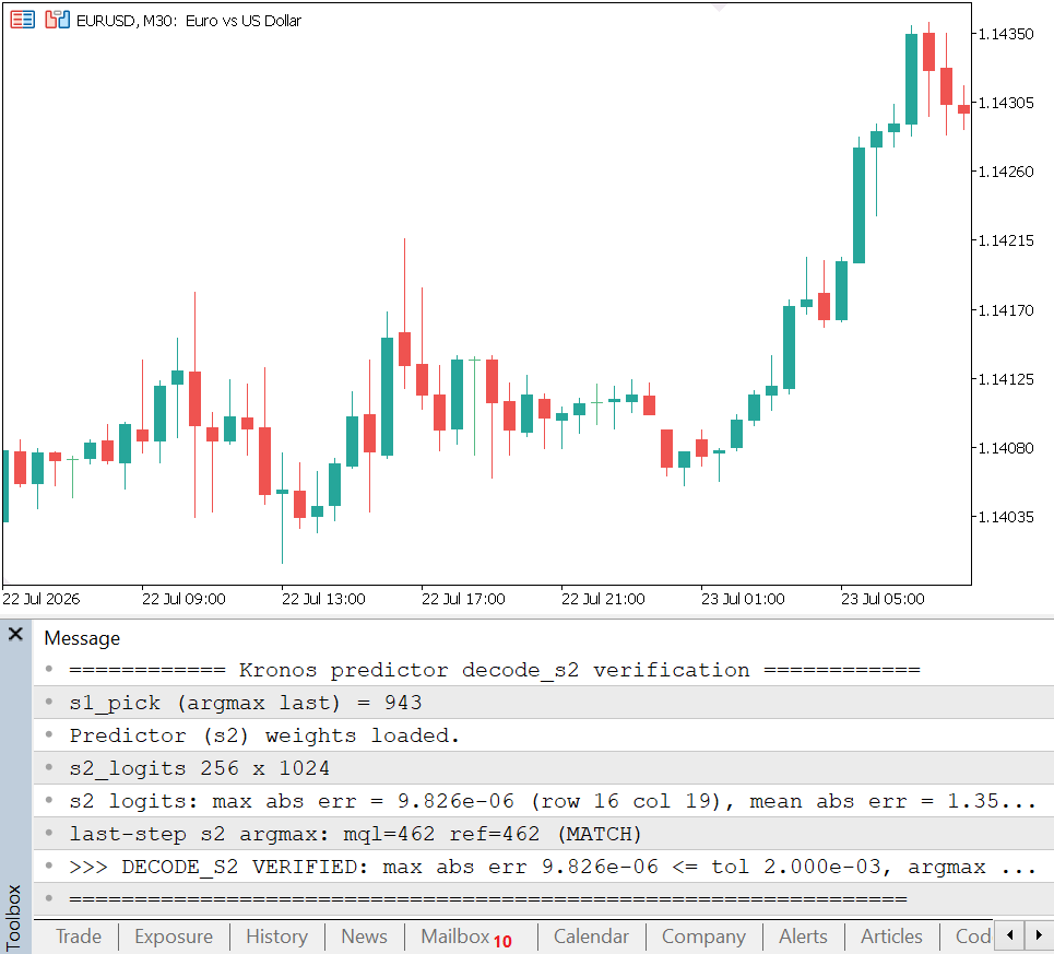
Fig. 5. The decode_s2 verification harness: with all three cross-attention traps handled, the s2 logits match the reference to about 9.8e-06 and the fine-token argmax agrees exactly (mql=462, ref=462)

Sampling the Next Token

Both decode_s1 and decode_s2 hand back a 1024-way logit vector, not a token. Turning a logit vector into an actual token id is the job of the sampling layer, and it is more than an argmax: the same four controls that the reference exposes, temperature, top-k, top-p, and a greedy switch, live in KronosSampling.mqh. They are worth understanding in full, because Part 3's evaluation runs the model in greedy mode for reproducibility, while any real deployment would sample, and the difference is entirely in this file.

The filtering step is the subtle part. Top-k keeps only the k highest logits; top-p (nucleus sampling) keeps the smallest set of tokens whose probabilities sum past a threshold. The trap in top-p is the boundary token, the one that tips the cumulative sum over the threshold. It must be kept, not dropped, otherwise the nucleus is one token too small. The implementation computes a removal mask from the cumulative sum and then shifts it by one position. This keeps the boundary token that crosses the threshold:

//+------------------------------------------------------------------+
//| Top-k then top-p filtering. Removed logits are set to -inf, at   |
//| least one token is kept, and the first token that crosses the    |
//| cumulative top-p threshold is itself kept.                       |
//+------------------------------------------------------------------+
void TopKTopPFilter(double &logits[], int top_k, double top_p)
  {
   int n = ArraySize(logits);

   if(top_k > 0)
     {
      int k = (int)MathMin(MathMax(top_k, 1), n);
      double tmp[];
      ArrayCopy(tmp, logits);
      int order[];
      ArgsortDesc(tmp, order);
      double kth = logits[order[k - 1]];
      for(int i = 0; i < n; i++)
         if(logits[i] < kth)
            logits[i] = KR_NEG_INF;
     }

   if(top_p < 1.0)
     {
      int order[];
      ArgsortDesc(logits, order);
      double probs[];
      ArrayResize(probs, n);
      for(int i = 0; i < n; i++)
         probs[i] = logits[order[i]];
      Softmax(probs);

      bool remove_sorted[];
      ArrayResize(remove_sorted, n);
      double cum = 0.0;
      for(int i = 0; i < n; i++)
        {
         cum += probs[i];
         remove_sorted[i] = (cum > top_p);
        }
      for(int i = n - 1; i > 0; i--)
         remove_sorted[i] = remove_sorted[i - 1];
      remove_sorted[0] = false;

      for(int i = 0; i < n; i++)
         if(remove_sorted[i])
            logits[order[i]] = KR_NEG_INF;
     }
  }

Removed tokens are set to a large negative sentinel rather than deleted, so the array keeps its vocabulary indexing; the matching Softmax maps those entries to zero probability. The final SampleFromLogits ties the controls together in the order the reference uses, divide by temperature, filter, softmax, then either take the argmax or draw:

//+------------------------------------------------------------------+
//| Full decode step: temperature scale, top-k/top-p filter,         |
//| softmax, then sample. greedy=true returns the argmax instead.    |
//+------------------------------------------------------------------+
int SampleFromLogits(const double &logits_in[], double T, int top_k, double top_p, bool greedy)
  {
   double l[];
   ArrayCopy(l, logits_in);
   int n = ArraySize(l);
   for(int i = 0; i < n; i++)
      l[i] /= T;
   if(top_k > 0 || top_p < 1.0)
      TopKTopPFilter(l, top_k, top_p);
   double probs[];
   ArrayCopy(probs, l);
   Softmax(probs);
   return greedy ? Argmax(probs) : MultinomialDraw(probs);
  }

Temperature T divides the logits before the softmax: below one it sharpens the distribution toward the top token, above one it flattens it. The greedy branch bypasses randomness entirely and returns the most probable token, which makes a whole forecast deterministic and reproducible. That determinism is what lets us verify generation against a fixed reference and what makes the Part 3 evaluation repeatable. The non-greedy branch calls MultinomialDraw, a plain inverse-CDF draw over the filtered distribution. This is the one place in the whole pipeline that is deliberately not bit-reproducible against PyTorch, which is exactly why verification is done greedily.

The Autoregressive Loop

We now have all four building blocks: encode a window to tokens, decode_s1 to predict a coarse token, decode_s2 to predict the fine token conditioned on it, and decode tokens back to candles. The autoregressive loop, inside GeneratePathNorm, wires them into a forecast. For each future bar it predicts the coarse token, samples it, predicts the fine token conditioned on that choice, samples it, and appends the new pair to the running sequence. Picking up right after decode_s1 has produced s1_logits for the step, the heart of one iteration is:

for(int i = 0; i < pred_len; i++)
  {
   //--- ... decode_s1 for this step fills s1_logits, context and last (next section) ...
   double l1[];
   ArrayResize(l1, (int)s1_logits.Cols());
   for(int j = 0; j < (int)s1_logits.Cols(); j++)
      l1[j] = s1_logits[last][j];
   int s1_pick = SampleFromLogits(l1, T, top_k, top_p, greedy);
   //--- decode_s2(context, [s1_pick]) -> sample last-step s2. The cross-attn
   //--- query (the single s1 pick) attends over the FULL context, so we pass
   //--- the whole context and read its last row.
   int pick_arr[];
   ArrayResize(pick_arr, 1);
   pick_arr[0] = s1_pick;
   matrix s2_logits;
   if(!m_p2.DecodeS2(context, pick_arr, s2_logits))
      return false;
   int s2_last = (int)s2_logits.Rows() - 1;
   double l2[];
   ArrayResize(l2, (int)s2_logits.Cols());
   for(int j = 0; j < (int)s2_logits.Cols(); j++)
      l2[j] = s2_logits[s2_last][j];
   int s2_pick = SampleFromLogits(l2, T, top_k, top_p, greedy);

   gen_s1[i] = s1_pick;
   gen_s2[i] = s2_pick;
   //--- append, sliding the buffer to max_context
   int n = ArraySize(pre);
   if(n < m_max_context)
     {
      ArrayResize(pre,  n + 1);
      pre[n]  = s1_pick;
      ArrayResize(post, n + 1);
      post[n] = s2_pick;
     }
   else
     {
      for(int t = 0; t < n - 1; t++)
        {
         pre[t] = pre[t + 1];
         post[t] = post[t + 1];
        }
      pre[n - 1]  = s1_pick;
      post[n - 1] = s2_pick;
     }
  }

Two things in this loop deserve attention. First, the single chosen s1 token is passed to decode_s2 as a one-element array, pick_arr, which is exactly the broadcast case the cross-attention traps were all about: one query, many keys, every key rotated at position zero. Because that query attends over the whole context, its output lands in the last row of s2_logits, which is the row the loop reads. Both picks come from the same SampleFromLogits we just built, so the greedy switch and the temperature/top-k/top-p controls apply identically to the coarse and fine tokens.

Second, the append is where the grow and slide phases live. While the buffer is shorter than m_max_context, the new token pair is simply appended, the grow phase. Once the buffer is full, the branch shifts every element down by one and writes the new pair at the end, dropping the oldest token so the window stays a fixed size, the slide phase. That branch looks like a housekeeping detail, but it is the exact hinge the KV-cache turns on: the cache is valid only in the first branch.

After the loop finishes, the full token sequence, context plus generated, is handed to the decoder, and the last pred_len reconstructed bars are the forecast. That whole path, generate then decode, is one sampled trajectory, and GeneratePathNorm produces exactly one. The public entry point, Predict, wraps it with the two steps that make it usable, normalization on the way in and averaging on the way out:

//+---------------------------------------------------------------+
//| Full predict: a raw OHLCVA window (L,6) plus stamps becomes a |
//| forecast (pred_len,6) in raw units. full_stamp is             |
//| (L+pred_len, 5) covering context and horizon, weekday in the  |
//| pandas convention. Averages sample_count paths in normalized  |
//| space (as the reference does), then denormalizes once.        |
//+---------------------------------------------------------------+
bool              Predict(const matrix &raw, const matrix &full_stamp, int pred_len,
              double T, int top_k, double top_p, int sample_count, bool greedy,
              matrix &forecast)
  {
   matrix x_norm;
   vector mean, stdv;
   KronosNormalize(raw, x_norm, mean, stdv);

   matrix avg = matrix::Zeros((ulong)pred_len, KR_NFEAT);
   int got = 0;
   for(int s = 0; s < sample_count; s++)
     {
      matrix p;
      int g1[], g2[];
      if(!GeneratePathNorm(x_norm, full_stamp, pred_len, T, top_k, top_p, greedy, p, g1, g2))
         return false;
      avg += p;
      got++;
     }
   if(got == 0)
      return false;
   avg *= (1.0 / (double)got);
//--- denormalize with the context window's per-feature stats
   KronosDenormalize(avg, mean, stdv, forecast);
   return true;
  }

The averaging is deliberately done in normalized space, matching the reference: each of the sample_count paths is a full generated trajectory, they are summed and divided, and only the mean is denormalized, once, with the context window's own statistics. This is why sampling can be noisy without wrecking the forecast, several draws smooth each other out. In greedy mode every path is identical, so sample_count is effectively one and the result is deterministic, which is the mode Part 3's evaluation uses. This method is the entire public surface of the engine: a raw OHLCVA window and its stamps go in, a forecast in real price units comes out, and everything in these two parts sits behind it.

Fig. 6. The autoregressive loop: each step predicts and samples the coarse then the fine token, appends them, and slides the window once it reaches the maximum context length

The slide branch is itself verified. A dedicated harness, KronosVerifyInference, drives greedy generation and checks the step-one tokens against the verified argmaxes (Fig. 7), while KronosVerifySlide pushes generation past the maximum context boundary and confirms that the tokens produced through the crossing match the reference exactly, 30 of 30, so the windowing logic is not just plausible but proven.

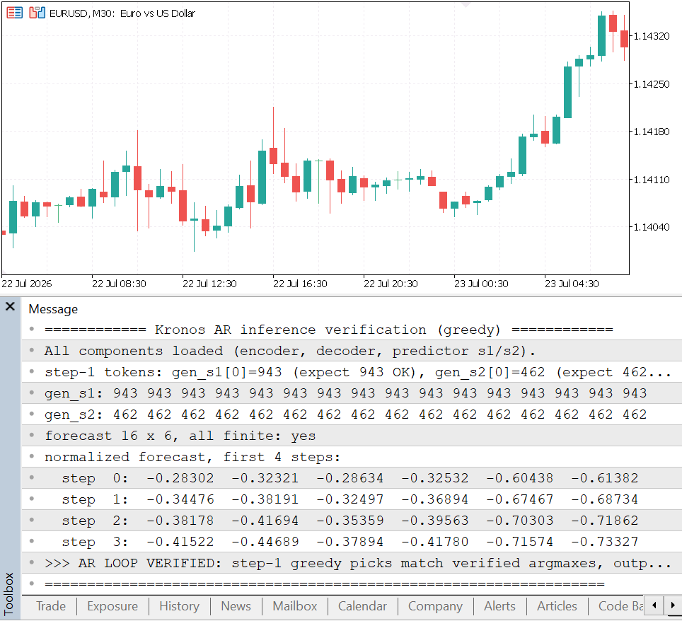
Fig. 7. The full autoregressive loop verified greedily: the step-one coarse and fine tokens (943 and 462) match the verified argmaxes, and the generated forecast is finite across all sixteen steps

A KV-Cache That Stays Exact

The loop above, written naively, is wasteful. At every step it re-runs all eight transformer blocks over the entire token window, even though only the last token is new. Everything the previous positions computed is thrown away and recomputed. That is the classic place a key/value cache helps: store each block's projected keys and values for the positions already seen, and at each step compute only the new row, attending it against the cache. The work per step drops from quadratic in the sequence length to linear.

What makes this model's cache tricky is rotary position embedding. RoPE bakes a token's absolute position into its key at the moment the key is rotated, so a cached key is only valid while that position never changes. That holds during the grow phase, when new tokens are appended to the end and nothing shifts. But the instant the window starts to slide, every surviving token's position drops by one and every cached key is stale. So the rule the implementation follows is: cache while it is exact, and fall back to the full recompute the moment it would not be.

The cache needs one primitive Part 1 did not: a RoPE application that rotates a whole multi-head row at an arbitrary absolute position offset, because the cached step rotates a single new row sitting at position pos, not at position 0. RoPEAllHeads is that primitive. It slices each head out, rotates it using the cos/sin row for posOffset + r, and writes it back:

//+---------------------------------------------------------------+
//| Apply RoPE per head over a (T, d_model) projection, using a   |
//| cos/sin table of width head_dim. Rotates each head's column   |
//| slice independently, matching MHA's per-head ApplyRoPE.       |
//| posOffset shifts the row->position mapping (row r uses        |
//| position posOffset+r) so a single appended row can be rotated |
//| at its true absolute position.                                |
//+---------------------------------------------------------------+
matrix            RoPEAllHeads(const matrix &M, const matrix &cosT, const matrix &sinT, int posOffset)
  {
   ulong T = M.Rows();
   ulong hd = m_dm / (ulong)m_heads;
   matrix outM = matrix::Zeros(T, m_dm);
   for(int h = 0; h < m_heads; h++)
     {
      ulong c0 = (ulong)h * hd;
      matrix Ms = SliceCols(M, c0, hd);
      //--- rotate slice; cos/sin row for output row r comes from posOffset+r
      matrix Mr = matrix::Zeros(T, hd);
      ulong half = hd / 2;
      for(ulong r = 0; r < T; r++)
        {
         ulong p = (ulong)posOffset + r;
         for(ulong k = 0; k < hd; k++)
           {
            double rh = (k < half) ? -Ms[r][k + half] : Ms[r][k - half];
            Mr[r][k] = Ms[r][k] * cosT[p][k] + rh * sinT[p][k];
           }
        }
      WriteCols(outM, Mr, c0);
     }
   return outM;
  }

Priming. Before generation begins, PrimeCache runs the initial context window through the eight blocks once. It cannot simply call TransformerBlock, because it needs to reach inside each block and capture the exact tensors attention forms, the post-RoPE keys and the raw values. So it re-implements the block body, and at the point where the keys are rotated it stores them:

for(int b = 0; b < m_blocks; b++)
  {
   //--- pre-norm + projections (mirrors MHA on RMSNorm(x))
   matrix n1 = RMSNorm(x, m_n1[b]);
   matrix Q  = LinearT(n1, m_Wq[b]);
   AddRowBias(Q, m_bq[b]);
   matrix K  = LinearT(n1, m_Wk[b]);
   AddRowBias(K, m_bk[b]);
   matrix V  = LinearT(n1, m_Wv[b]);
   AddRowBias(V, m_bv[b]);
   //--- RoPE the full Q and K per head at their own positions (posOffset 0)
   matrix Qr = RoPEAllHeads(Q, cosT, sinT, 0);
   matrix Kr = RoPEAllHeads(K, cosT, sinT, 0);
   //--- cache the post-RoPE K and raw V for this block
   m_cacheK[b] = Kr;
   m_cacheV[b] = V;
   //--- attention per head (causal), then out-proj + residual + FFN
   matrix ctx = matrix::Zeros((ulong)L, m_dm);
   for(int h = 0; h < m_heads; h++)
     {
      ulong c0 = (ulong)h * hd;
      matrix Qh = SliceCols(Qr, c0, hd);
      matrix Kh = SliceCols(Kr, c0, hd);
      matrix Vh = SliceCols(V,  c0, hd);
      matrix Oh = SDPA(Qh, Kh, Vh, true);   // causal, matches MHA
      WriteCols(ctx, Oh, c0);
     }
   matrix a = LinearT(ctx, m_Wo[b]);
   AddRowBias(a, m_bo[b]);
   matrix x1 = x + a;
   matrix n2 = RMSNorm(x1, m_n2[b]);
   matrix f  = SwiGLU(n2, m_W1[b], m_W3[b], m_W2[b]);
   x = x1 + f;
  }

After the prime, m_cacheK[b] and m_cacheV[b] hold the keys and values for every context position, per block, and a parallel m_cacheContext holds the post-final-norm context that decode_s2 will need. This is a deliberate mirror of the ordinary block, not a shortcut: the causal SDPA call and the residual/FFN wiring are identical to MHA and TransformerBlock, which is why the primed result is bit-for-bit the same as a full DecodeS1 over the same window.

Stepping. Each grow-phase step then does the cheap thing. DecodeS1Step embeds only the single new token, and for each block projects just that one row, rotates it at its own absolute position pos, appends its key and value to the cache, and attends the one new query against the whole stored history:

int pos = m_cacheLen;             // absolute position of the new row
ulong hd = m_dm / (ulong)m_heads;
//--- RoPE table sized to cover position `pos` (rows 0..pos), query reads row pos
matrix cosT, sinT;
RoPETables((ulong)(pos + 1), hd, cosT, sinT);

for(int b = 0; b < m_blocks; b++)
  {
   matrix n1 = RMSNorm(x, m_n1[b]);          // (1, d_model)
   matrix Q  = LinearT(n1, m_Wq[b]);
   AddRowBias(Q, m_bq[b]);
   matrix K  = LinearT(n1, m_Wk[b]);
   AddRowBias(K, m_bk[b]);
   matrix V  = LinearT(n1, m_Wv[b]);
   AddRowBias(V, m_bv[b]);
   //--- rotate the single new row at its absolute position `pos`
   matrix Qr = RoPEAllHeads(Q, cosT, sinT, pos);
   matrix Kr = RoPEAllHeads(K, cosT, sinT, pos);
   //--- append new K/V to the cache for this block -> (pos+1, d_model)
   matrix Kall = AppendRow(m_cacheK[b], Kr);
   matrix Vall = AppendRow(m_cacheV[b], V);
   m_cacheK[b] = Kall;
   m_cacheV[b] = Vall;
   //--- attention: single query (row pos) over all cached keys (non-causal:
   //--- the new row is the latest position, so it attends to everything)
   matrix ctx = matrix::Zeros(1, m_dm);
   for(int h = 0; h < m_heads; h++)
     {
      ulong c0 = (ulong)h * hd;
      matrix Qh = SliceCols(Qr,   c0, hd);   // (1, hd)
      matrix Kh = SliceCols(Kall, c0, hd);   // (pos+1, hd)
      matrix Vh = SliceCols(Vall, c0, hd);
      matrix Oh = SDPA(Qh, Kh, Vh, false);   // (1, hd)
      WriteCols(ctx, Oh, c0);
     }
   matrix a  = LinearT(ctx, m_Wo[b]);
   AddRowBias(a, m_bo[b]);
   matrix x1 = x + a;
   matrix n2 = RMSNorm(x1, m_n2[b]);
   matrix f  = SwiGLU(n2, m_W1[b], m_W3[b], m_W2[b]);
   x = x1 + f;
  }

The attention here is marked non-causal, which is correct precisely because the new row is the latest position: it is allowed to see every earlier key, and there is nothing later to mask. The keys it reads were each rotated at their own position when they were first cached, so the single new query, rotated at pos, sees a history that is positionally consistent with what a full recompute would have built. The cache also grows m_cacheContext by the new row, because decode_s2's cross-attention still reads across all positions, not just the last.

The whole scheme is gated on staying in the grow phase. The autoregressive loop decides, per step, whether the cache is still exact and uses it only then:

//--- decode_s1: cached grow-phase step, or full-window fallback
matrix s1_logits, context;
int last;
bool use_cache = (cache_ok && current_seq_len < m_max_context);

While current_seq_len is below the maximum context, the loop takes the cached step; once the window would slide, use_cache goes false and it calls the full, untouched DecodeS1 over the current window instead. Correctness is never traded for speed: the cached and full logits agree to about 1e-14, and every generation harness, including the slide test, passes unchanged with the cache in place. This is the single largest piece of engineering in the port, and it is the reason a multi-bar forecast finishes in seconds rather than minutes.

Fig. 8. The cache lifecycle. PrimeCache fills the per-block K/V over the whole context once; each grow-phase step projects and rotates only the new row and appends it; the instant the window would slide, the loop drops the cache and falls back to a full DecodeS1 recompute

Making It Fast: Profiling and Pre-Transposed Weights

The KV-cache was the first speedup, and an obvious one: it removes work the model was doing redundantly. The second speedup was not obvious at all, and it is the more instructive story, because it came from measurement contradicting intuition.

Even with the cache, the first end-to-end version was slow. Generating a single forecast at a 256-bar context took on the order of nine hundred milliseconds per step, which makes a walk-forward study over thousands of bars impractical. The temptation at this point is to guess at the bottleneck and start optimizing. We profiled instead, with a headless one-shot driver, KronosProfile.mq5, that runs a single Predict under the MetaEditor profiler. Running Predict as a script rather than inside the visualization-only EA matters here, because the EA hangs under the profiler; the script form gives a clean one-shot pass to measure. The profiler said something surprising.

The biggest single cost was transposing weights. The linear layer, as first written, transposed its weight matrix on every call to match the PyTorch convention. Because that weight is constant, the same transpose was being recomputed thousands of times, and it added up to roughly sixty percent of the entire forward pass. The fix costs nothing at runtime: store every linear weight already transposed, once, at load time. We met this in Part 1, the KronosLoadMatrixT loader and the one-line LinearT, and this is the measurement that motivated it. The math is identical; the transpose simply moves from every call to a single load.

The two fixes compound: the cache from the previous section and the transpose fix here. A small timing script, KronosBench.mq5, measures the per-step latency at a given context length, and the table shows the measured per-step time at a 256-bar context, greedy, single path:

Build	Per-step time	Speedup
Pre-cache baseline	~906 ms	1.0x
+ grow-phase KV-cache	~423 ms	~2.1x
+ pre-transposed weights	~201 ms	~4.5x

That is roughly a four and a half times cumulative speedup. The table isolates a single greedy step so the two fixes can be compared cleanly; a real forecast is heavier, since it runs several sampled paths to their full length. Profiling one such realistic run, sixteen bars ahead with five sampled paths, shows the end-to-end cost: about 17.5 seconds total, roughly 220 milliseconds per step per path, down from what would have been well over a minute before these two fixes. After the transpose fix the profile is flat, with no single dominant cost: the real matrix multiply is the legitimate floor, and the rest is split among data-shuffling, the elementwise normalization and activation loops, and sampling. There are further levers available, float32 arithmetic, batching the sample paths, OpenCL, but none is pursued blindly. The lesson the profiler taught, that the bottleneck was not where intuition pointed, is the one worth keeping.

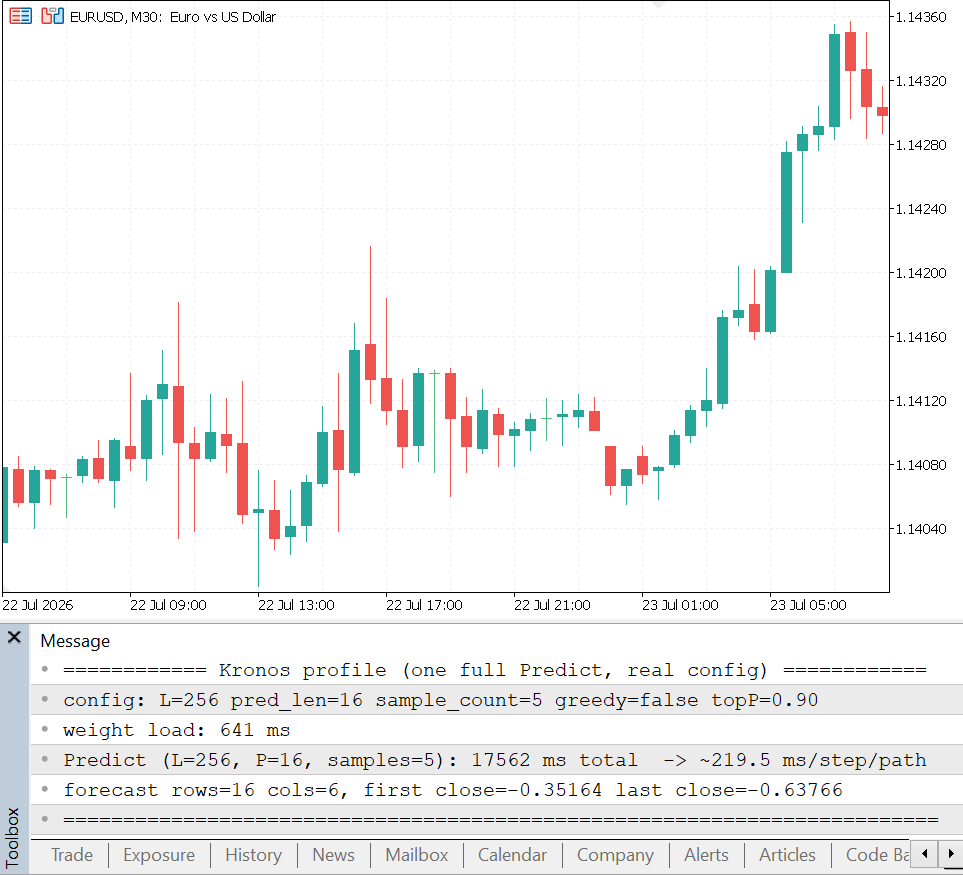
Fig. 9. A single full Predict profiled at the real configuration (256-bar context, sixteen bars ahead, five sampled paths): about 17.5 seconds total, roughly 220 milliseconds per step per path, after both the KV-cache and the pre-transposed-weights fixes

Note: the key/value cache is exact only while the context window grows, because rotary embeddings encode absolute position into each key. Once the window slides, positions shift and the cache is dropped in favor of the full recompute. Speed is never bought at the cost of a wrong number.

Conclusion

The pipeline is now complete and verified end to end. We built the decoder that turns tokens back into candles, the predictor's hierarchical embedding, the decode_s1 and decode_s2 stages with their cross-attention dependency, and the autoregressive loop that produces a multi-bar forecast. Then we profiled the result and made it roughly four and a half times faster without changing a single output.

• The traps are concentrated and subtle. The full-vs-reduced block count, the unscaled sibling embedding, the four-head cross-attention, and the query-length rotary cache each produced output that looked right while being wrong.
• The cache is exact, not approximate. It is used only in the grow phase where absolute positions are stable, and the loop falls back to a full recompute the instant the window slides.
• Profile before optimizing. The dominant cost was a constant weight transpose being recomputed thousands of times, not anywhere intuition would have looked first.
• Every stage is pinned to a reference. Decoder around 1.8e-06, s1 around 4.7e-06, s2 around 9.8e-06, the slide branch exact, the cache exact to 1e-14.

We have exhaustively verified that the MQL5 port reproduces Kronos faithfully. That is a statement about fidelity to PyTorch, and it is the only thing verification can establish. It is worth being precise about what it does and does not claim: it means the engine computes what the original model computes, not that the original model's forecasts are any good in the market. Those are two separate questions, and conflating them is a trap the next part is written to avoid. The pipeline built and verified across these two parts is the tool that makes an honest answer possible; Part 3 puts it to work in a look-ahead-safe walk-forward evaluation.

The programs presented in this article are intended for educational purposes only. They demonstrate a porting, verification, and optimization methodology, not a trading recommendation. Whether the model's forecasts carry any usable edge is evaluated separately in Part 3. Past performance and model fidelity do not guarantee future results.

Getting the Source Code via MQL5 Algo Forge

All source files are attached to this article below, but the full repository is also available on MQL5 Algo Forge, the community's Git-based platform for sharing and collaborating on trading projects. 

File name	Description
MQL5\Include\Kronos\KronosDecoder.mqh	CKronosDecoder: the tokenizer decode chain from token ids back to a normalized OHLCVA window
MQL5\Include\Kronos\KronosPredictorS1.mqh	CKronosPredictorS1: hierarchical and temporal embedding, decode_s1, and the grow-phase KV-cache (PrimeCache / DecodeS1Step)
MQL5\Include\Kronos\KronosPredictorS2.mqh	CKronosPredictorS2: decode_s2 with the dependency-aware cross-attention head
MQL5\Include\Kronos\KronosSampling.mqh	Sampling utilities: softmax, top-k and top-p filtering, multinomial draw, and greedy selection
MQL5\Include\Kronos\KronosInference.mqh	CKronosModel: the autoregressive loop, sample-path averaging, and the full Predict entry point
MQL5\Scripts\Kronos\KronosVerifyDecoder.mq5	Golden-reference harness for the decoder reconstruction
MQL5\Scripts\Kronos\KronosVerifyPredictorS1.mq5	Golden-reference harness for the decode_s1 logits
MQL5\Scripts\Kronos\KronosVerifyPredictorS2.mq5	Golden-reference harness for the decode_s2 logits
MQL5\Scripts\Kronos\KronosVerifySlide.mq5	Golden-reference harness for the slide-phase token generation past the context boundary
MQL5\Scripts\Kronos\KronosVerifyInference.mq5	Golden-reference harness for the autoregressive loop: greedy step-one tokens against the verified argmaxes
MQL5\Scripts\Kronos\KronosBench.mq5	Timing script that measures per-step forecast latency at a given context length
MQL5\Scripts\Kronos\KronosProfile.mq5	Headless one-shot Predict() entry point used to drive the MQL5 profiler
MQL5\Kronos\kronos_slide_capture.py	Offline, one-time: captures the long-context greedy slide reference used by the slide-phase harness