Overcoming The Limitation of Machine Learning (Part 5): A Quick Recap of Time Series Cross Validation

In our related series of articles, we’ve covered numerous tactics on how to deal with issues created by market behavior. However, in this series, we focus on problems caused by the machine learning algorithms we wish to employ in our strategies. Many of these issues arise from the architecture of the model, the algorithms used in model selection, the loss functions we define to measure performance, and many other subjects of the same nature.

All the moving parts that collectively build a machine learning model, may unintentionally create obstacles in our pursuit of applying machine learning to algorithmic trading requiring careful diagnostic assessment. Therefore, it is important for each of us to understand these limitations and, as a community, build new solutions and define new standards for ourselves.

Machine learning models used in algorithmic trading face unique challenges, often caused by the way we validate and test them. One critical step is time series cross-validation — a method for evaluating model performance on unseen, chronologically ordered data.

Unlike standard cross-validation, time series data cannot be shuffled, as that would leak future information into the past. This makes resampling more complex and introduces unique trade-offs between bias, variance, and robustness.

In this article, we introduce cross-validation for time series, explain its role in preventing overfitting, and show how it can help train reliable models even on limited data. Using a small two-year dataset, we demonstrate how proper cross-validation improved the performance of a deep neural network compared to a simple linear model.

Our goal is to highlight both the value and limitations of common time series cross-validation methods, laying the foundation for a deeper discussion in the next part of the series.

Fetching Data in MQL5

For this discussion, we begin by fetching historical data from the MetaTrader 5 terminal using an MQL5 script that we wrote by hand. The script starts by saving the name of the file that will be written out.

Next, we store the amount of data to be fetched as an input parameter that the user can pass to the script. Be sure to set the property #property script_show_inputs in the header of your script to ensure the end user is able to specify the number of bars to fetch.

After gathering all the necessary information, we initiate the process of writing the file. Using the FileOpen function, we create a new file handler. This function accepts parameters that define the type of file being used, the operations to be performed on it, and the delimiter or spacing convention for the file.

Therefore, we pass the FileOpen method the file name generated at the beginning of the script, the appropriate file operation modes and types, and the comma as our delimiter of choice.

After that, we initialize a for loop that runs from the total number of bars to be fetched down to the beginning. In the first iteration, we write out the column names that we want to store in our CSV file. For each subsequent iteration, we fetch the relevant market data corresponding to that point in time, moving gradually from the past toward the present.

This ensures that our CSV file is structured with the oldest dates at the top and the most recent dates toward the end.

//+------------------------------------------------------------------+
//|                                                      Fetch_Data  |
//|                                      Copyright 2020, CompanyName |
//|                                       http://www.companyname.net |
//+------------------------------------------------------------------+
#property copyright "Copyright 2024, MetaQuotes Ltd."
#property link      "https://www.mql5.com"
#property version   "1.00"
#property script_show_inputs

//--- File name
string file_name = Symbol() + " Detailed Market Data As Series.csv";

//--- Amount of data requested
input int size = 3000;

//+------------------------------------------------------------------+
//| Our script execution                                             |
//+------------------------------------------------------------------+
void OnStart()
  {
   int fetch = size;

//---Write to file
   int file_handle=FileOpen(file_name,FILE_WRITE|FILE_ANSI|FILE_CSV,",");

   for(int i=size;i>=1;i--)
     {
      if(i == size)
        {
         FileWrite(file_handle,"Time",
                   //--- OHLC
                   "True Open",
                   "True High",
                   "True Low",
                   "True Close"
                  );
        }

      else
        {
         FileWrite(file_handle,
                   iTime(_Symbol,PERIOD_CURRENT,i),
                   //--- OHLC
                   iClose(_Symbol,PERIOD_CURRENT,i),
                   iOpen(_Symbol,PERIOD_CURRENT,i),
                   iHigh(_Symbol,PERIOD_CURRENT,i),
                   iLow(_Symbol,PERIOD_CURRENT,i)
                  );
        }
     }
//--- Close the file
   FileClose(file_handle);
  }
//+------------------------------------------------------------------+

Analyzing Our Data In Python

After successfully writing out our CSV file, the next step is to import our Pandas, NumPy, and Matplotlib libraries in order to get started with our analysis. 

#Import basic libraries
import pandas as pd
import numpy as np
import matplotlib.pyplot as plt

When reading the data created using the MQL5 script, note that in the example code below, the reader should replace the path with their own system path.

#Read in the data
data = pd.read_csv("/ENTER/YOUR/PATH/HERE/EURUSD Detailed Market Data As Series.csv")

In our example, we want to demonstrate that cross-validation can be used to fit complex models even with limited datasets. Therefore, we will select the last two years of data and drop everything else.

data = data.iloc[(365*2):,:]
data.reset_index(drop=True,inplace=True)

From there, we must define how far into the future we wish to forecast. 

#Define a forecast horizon
HORIZON  = 1

Next step is to prepare the inputs we want to work with — the differenced inputs. We create these by subtracting the current input from its previous value. We also add the label to the dataset. After that, we drop all missing values.

#Let us start by following classical rules
data['True Close Diff'] = data['True Close'] - data['True Close'].shift(HORIZON)
data['True Open Diff'] = data['True Open'] - data['True Open'].shift(HORIZON)
data['True High Diff'] = data['True High'] - data['True High'].shift(HORIZON)
data['True Low Diff'] = data['True Low'] - data['True Low'].shift(HORIZON)

#Add the target
data['Target'] = data['True Close'] - data['True Close'].shift(-HORIZON)
data.dropna(inplace=True)
data.reset_index(inplace=True,drop=True)

Let us visualize the data.

#Let's visualize the data
plt.plot(data['True Close'],color='black')
plt.grid()
plt.title('EURUSD Data From 2023 - 2024')
plt.xlabel('Time')
plt.ylabel('EURUSD Exchange Rate')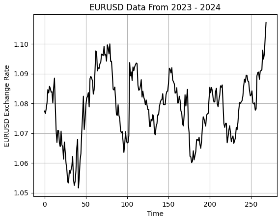

Figure 1: Visualizing our small sample of historical EURUSD exchange rates

Next, we partition our dataset into two halves: the first half for training and the latter for testing.

#Partition the data
train , test = data.iloc[:data.shape[0]//2,:] , data.iloc[data.shape[0]//2:,:]

Store the inputs and targets separately.

#Differenced inputs
X = train.iloc[:,5:-4].columns
y = 'Target'

We now load our machine learning libraries and evaluation metrics to assess the models. 

#Load a machine learning library
from sklearn.neural_network import MLPRegressor
from sklearn.linear_model import LinearRegression,Ridge
from sklearn.metrics import root_mean_squared_error

As stated earlier in the introduction of this article, we first define a control setup by creating our linear model.

#Start the model
model   = Ridge(alpha=1e-7)

Fit the model.

model.fit(train.loc[:,X],train.loc[:,y])

Lastly, we store the predictions made by the model on the test set without fitting the model on that set. Recall that it is important not to fit the model on the test set, because we will use that portion of data later to evaluate our model during the backtest in MetaTrader 5.

test['Predictions'] = model.predict(test.loc[:,X])

Let us now generally assess how sound our model is. We begin by plotting the predictions our model made on the out-of-sample data and comparing them against the actual realized price levels. As we can see, when we plot the performance of our model, the model appears to have a reasonable understanding of the future behavior of price levels. The predictions it made appear coherent and align well with the real trajectory followed by the actual target. However, there are times we can also observe that the model does not capture the fluctuations in price data as effectively as we may desire. 

plt.plot(test.loc[:,'Target'],color='black')
plt.plot(test.loc[:,'Predictions'],color='red',linestyle=':')
plt.legend(['Target','Predictions'])
plt.title('Visualizing Model Accuracy Out of Sample')
plt.xlabel('Time')
plt.ylabel('EURUSD Exchange Rate')
plt.grid()

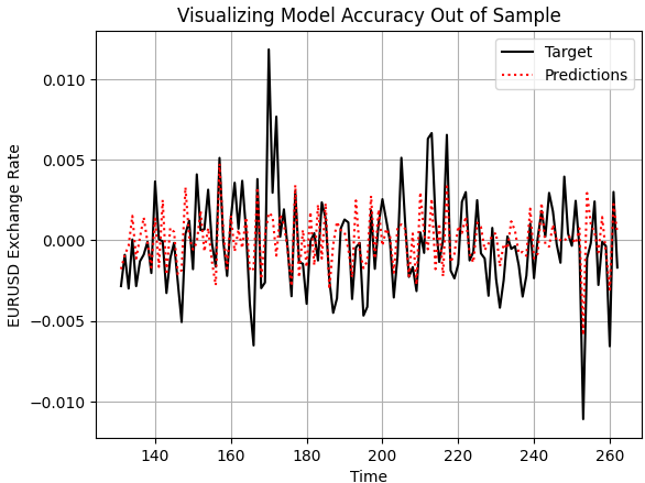
Figure 2: Visualizing the out of sample accuracy our simple linear model could achieve

Additionally, the correlation levels produced by our linear model and the real target are rather low. The model produces a correlation of 0.58, which is relatively poor.

test.loc[:,['Target','Predictions']].corr().iloc[0,1]

0.5826364163824712

Converting To ONNX

ONNX, which stands for Open Neural Network Exchange, is an open-source protocol that lets us build and deploy machine learning models across different frameworks. It’s language-agnostic, meaning we can train a model in one language that supports the ONNX API and export it to another for deployment, as long as both support ONNX. This allows the same model to be used across many systems.

All of this is possible thanks to the widespread adoption of the ONNX API. So, we begin by importing the ONNX library, along with a conversion library that turns scikit-learn models into their ONNX representations.An ONNX representation is simply a mathematical computation graph that describes the model. This graph can easily be converted back into the original implementation.

import onnx
from skl2onnx import convert_sklearn
from skl2onnx.common.data_types import FloatTensorType

Once the ONNX library is imported, we define the input and output shapes that the model accepts and returns. 

initial_types = [("FLOAT INPUT",FloatTensorType([1,4]))]
final_types = [("FLOAT OUTPUT",FloatTensorType([1,1]))]

We then convert each of our trained models into their ONNX prototypes.

model_proto = convert_sklearn(model,initial_types=initial_types,target_opset=12)
model2_proto = convert_sklearn(model2,initial_types=initial_types,target_opset=12)

Next, we save these prototypes as .onnx files using the ONNX save method. 

onnx.save(model_proto,"EURUSD LR D1 DIFFERENCED.onnx")
onnx.save(model2_proto,"EURUSD LR 2 D1 RAW.onnx")

Defining Our Benchmark Performance Level

We begin by loading the ONNX buffer created earlier.

//-- Load the onnx buffer
#resource "\\Files\\EURUSD LR D1 DIFFERENCED.onnx" as const uchar onnx_buffer[];

Then, we define global variables related to the ONNX model, including prediction storage and model handlers.

//--- Global variables
long   onnx_model;
vector onnx_inputs,onnx_output;

After that, we load the Trade library, which helps us manage positions and risk levels.

//--- Libraries
#include <Trade\Trade.mqh>
CTrade Trade;

When the model is initialized for the first time, we prepare it with the OnnxCreateFromBuffer() method. This method takes two parameters:

1. The ONNX buffer created from file.

2. The initialization arguments—such as specifying the ONNX data type as float, since float inputs and outputs are stable and widely used in ONNX.

We then set the model’s input and output shapes to match those defined earlier in Python. 

//+------------------------------------------------------------------+
//| Expert initialization function                                   |
//+------------------------------------------------------------------+
int OnInit()
  {
//--- Prepare the ONNX model
onnx_model = OnnxCreateFromBuffer(onnx_buffer,ONNX_DEFAULT);

//--- Set the input shape of the model
ulong model_input[] = {1,4};
OnnxSetInputShape(onnx_model,0,model_input);

ulong model_output[] = {1,1};
OnnxSetOutputShape(onnx_model,0,model_output);
   
//---
   return(INIT_SUCCEEDED);
  }

When the application closes, we free the resources allocated to the ONNX model, which is good practice in MQL5.

//+------------------------------------------------------------------+
//| Expert deinitialization function                                 |
//+------------------------------------------------------------------+
void OnDeinit(const int reason)
  {
//--- Free up dedicated ONNX resources
OnnxRelease(onnx_model);
  }

Each time we receive new prices, we first check if there are no open positions. If that’s the case, we prepare to get a prediction from the ONNX model to decide what position to take.

To do this, we resize the input vector to match the expected shape—here, size four. Each input is processed and cast to the float type. We also fetch market data such as bid and ask prices. A variable called padding determines how wide our stop loss will be.

Next, we prepare a vector to store the model’s prediction—this should be of length one. We then use the OnnxRun() command to get a forecast, print it to the terminal, and compare it to the actual market price to generate a trading signal.

This is the classic way machine learning models are used in trading systems. If a position is already open, we simply wait for it to hit either the stop loss or take profit. This helps us evaluate how accurate and consistent the

//+------------------------------------------------------------------+
//| Expert tick function                                             |
//+------------------------------------------------------------------+
void OnTick()
  {
//--- Check if we have no open positions
if(PositionsTotal() ==0)
   {
      //--- Prepare the model inputs
      onnx_inputs.Resize(4);
      onnx_inputs[0] = (float) iClose(Symbol(),PERIOD_D1,0) - iClose(Symbol(),PERIOD_D1,1);
      onnx_inputs[1] = (float) iOpen(Symbol(),PERIOD_D1,0) - iOpen(Symbol(),PERIOD_D1,1);
      onnx_inputs[2] = (float) iHigh(Symbol(),PERIOD_D1,0) - iHigh(Symbol(),PERIOD_D1,1);
      onnx_inputs[3] = (float) iLow(Symbol(),PERIOD_D1,0) - iLow(Symbol(),PERIOD_D1,1);
      
      //--- Market data
      double ask = SymbolInfoDouble(Symbol(),SYMBOL_ASK);
      double bid = SymbolInfoDouble(Symbol(),SYMBOL_BID);
      double padding = 5e-3;
      
      //--- Store the model's prediction
      onnx_output.Resize(1);
      if(OnnxRun(onnx_model,ONNX_DATA_TYPE_FLOAT,onnx_inputs,onnx_output))
         {
            Print("Model forecast: ",onnx_output[0]);
            
            //--- Buy setup
            if(onnx_output[0] > iClose(Symbol(),PERIOD_D1,0)) Trade.Buy(0.01,Symbol(),ask,ask-padding,ask+padding,"");
            
            //--- Sell setup
            else if(onnx_output[0] <  iClose(Symbol(),PERIOD_D1,0)) Trade.Sell(0.01,Symbol(),bid,bid+padding,bid-padding,"");
         }
   }
   
//--- Otherwise, if we do have open positions
else if(PositionsTotal()>0)
   {
      //--- Then
      Print("Position Open");
   }
  }
//+------------------------------------------------------------------+

We begin, as usual, by highlighting the dates we reserved for our backtest. Recall that in Python, we partitioned our dataset in half and did not fit our model on the test set. These are the same dates we have selected for our MetaTrader 5 practice. This gives us a healthy benchmark to try outperforming using our deep neural network. 

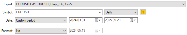
Figure 3: Selecting the dates we need for our control backtest

We will also select random delay settings to ensure that our back test conditions match real life trading conditions.

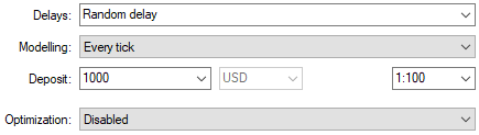
Figure 4: Select back test conditions that emulate expected deployment conditions

When we analyze the equity curve produced by the trading strategy, we can see that although the initial strategy got off to a slow start in the first half of the backtest period, it proved profitable in the end.

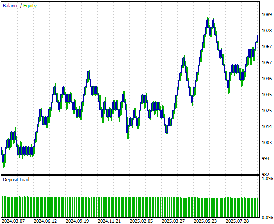
Figure 5: The equity curve produced by our simple linear model appears promising, but we can still reach to higher levels of performance

When we look at the detailed performance statistics, we can see there’s still room for improvement. For example, the model’s short entries perform particularly poorly—close to fifty percent accuracy, which is just slightly better than chance. However, it’s also interesting to note that the model appears well-founded on long entries. 

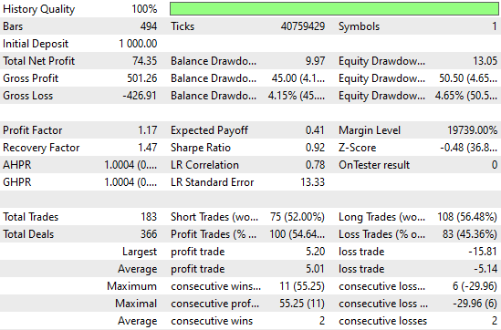
Figure 6: Visualizing the detailed statistics, we obtained from evaluating our simple Ridge model on out of sample data

Improving Our Initial Results

Now, let’s try to improve these initial results. We begin by importing the appropriate resampling methods from the scikit-learn library: RandomizedSearchCV and TimeSeriesSplit. These two can be used together for time series resampling.

from sklearn.model_selection import RandomizedSearchCV,TimeSeriesSplit

Next, we create a TimeSeriesSplit object with five folds, and set the gap between each fold equal to the forecasting horizon.

tscv = TimeSeriesSplit(n_splits=5,gap=HORIZON)

From there, we create a neural network with basic settings that will remain consistent across all iterations of our cross-validation tests.

nn = MLPRegressor(random_state=0,shuffle=False,early_stopping=False,max_iter=1000)

We also create a dictionary of parameters for our deep neural network. Each of these parameters will be tried and compared in order to identify the best model.

distributions = dict(activation=['identity','logistic','tanh','relu'],
                     alpha=[100,10,1,1e-1,1e-2,1e-3,1e-4,1e-5,1e-6,1e-7],
                     hidden_layer_sizes=[(4,40,20,10,2),(4,100,200,500,100,4),(4,20,40,20,4,2),(4,10,50,10,4),(4,4,4,4)],
                     solver=['adam','sgd','lbfgs'],
                     learning_rate = ['constant','invscaling','adaptive']
                     )

We then use the randomized search procedure, which performs a controlled number of iterations from all possible parameter combinations. It doesn’t search the entire input space exhaustively, but instead allows us to control how rigorous the search is by tuning the n_iter parameter.

rscv = RandomizedSearchCV(nn,distributions,random_state=0,n_iter=50,n_jobs=-1,scoring='neg_mean_squared_error',cv=tscv)

To perform the cross-validation, we simply call the fit() method on the RandomizedSearchCV object we created earlier, and store the results in a variable named after our neural network search procedure.

nn_search = rscv.fit(train.loc[:,X],train.loc[:,y])

After the search is complete, we retrieve the best parameters found by cross-validation. 

nn_search.best_params_

{'solver': 'lbfgs',

'learning_rate': 'adaptive',

'hidden_layer_sizes': (4, 40, 20, 10, 2),

'alpha': 0.0001,

'activation': 'identity'}

We then initialize a new model with these parameters and fit it on the training set.

model = MLPRegressor(random_state=0,shuffle=False,early_stopping=False,max_iter=1000,solver='lbfgs',learning_rate='adaptive',hidden_layer_sizes=(4, 40, 20, 10, 2),alpha=0.0001,activation='identity')

model.fit(train.loc[:,X],train.loc[:,y])

 Finally, we convert the model to its ONNX prototype.

model_proto = convert_sklearn(model,initial_types=initial_types,target_opset=12)

Finally, we save the ONNX file of the neural network to our drive so that we can test the improvements we’ve made.

onnx.save(model_proto,'EURUSD NN D1.onnx')

Implementing Our Improvements

Most parts of our previous application remain the same, so now we can focus on the few lines of code we need to update to reflect our improved model. The only line to change is the resource path in our header file—it must be updated to point to the new neural network model we just created.

//-- Load the onnx buffer
#resource "\\Files\\EURUSD NN D1.onnx" as const uchar onnx_buffer[];

Once that’s complete, we can observe how our new application performs over the same backtest period. We’ll select the same dates as before to ensure a fair comparison.

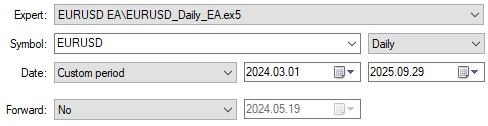
Figure 7: Selecting our new and improved deep neural network application to trade over the same test period

When we analyze the detailed performance statistics, we can already see notable changes. The total net profit has grown materially along with the number of trading signals registered by the system. This means the neural network has increased profitability while placing more trades than the previous version—at consistent accuracy levels. These are quite impressive improvements to observe.

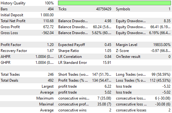
Figure 8: Our performance levels have improved considerably over the control bench mark we established

Finally, when we look at the equity curve produced by the new version of the application, we can clearly see that the consolidation period which previously stagnated growth in our initial backtest has now been replaced by a strong, explosive upward trend created by our neural network. This gives us a more reliable and robust source of trading signals moving forward.

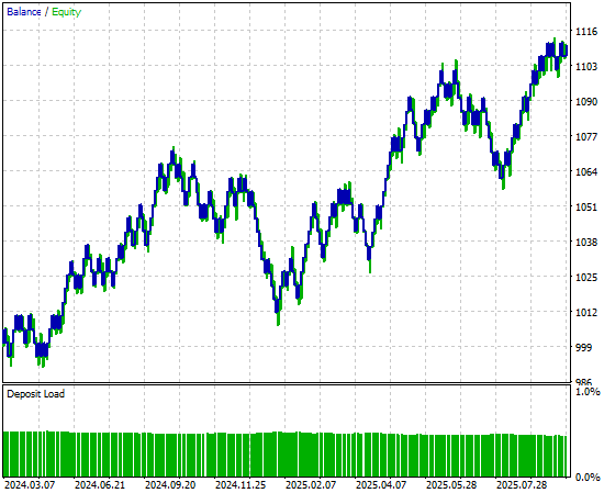
Figure 9: Visualizing the equity curve produced by our strategy, that we improved using time series cross validation

Conclusion

This article has given the reader an overview of the strengths of time series cross-validation techniques when they are applied meaningfully. The reader walks away knowing that time series cross-validation can be used to help mitigate the risk of overfitting, tune and search for better model parameters, identify the best possible method from a pool of candidate models, and estimate the test error of a model on data it has not yet seen.

As we have repeated throughout this article, this list of use cases is by no means exhaustive. It would be impossible to cover all the advantages that time series cross-validation brings to our modeling pipeline.

However, now that we have reached this point in our discussion, the reader should be well prepared to question more deeply. Can the performance levels we have demonstrated here today can still be improved using more rigorous forms of time series cross-validation than the simple K-Fold method presented here? These are questions definitely worthwhile to explore further.

In the following discussions, we will consider alternative cross-validation methods, such as Walk-Forward Time Series Cross-Validation, and contrast them to the K-Fold approach. Through this comparison, we will learn how to reason why one method may be more appropriate than another. And for you to understand when that might apply, you must first have a clear idea of what good cross-validation can do for you.

File Name	File Description
Fetch_Data.mq5	The custom MQL5 script we wrote to fetch our historical data from the MetaTrader 5 Terminal.
The_Limitations_of_AI_Model_Selection.ipynb	The JupyterNotebook we wrote to analyze the market data we retreived from the MetaTrader 5 Terminal.
EURUSD_LR_D1_DIFFERENCED.onnx	The linear regression ONNX model we created as our benchmark model.
EURUSD_NN_D1.onnx	The deep neural network ONNX model we created to surpass the benchmark.
EURUSD_Daily_EA.mq5	The deep neural network enhanced trading application we optimized using time series cross validation.
EURUSD_Daily_EA_3.mq5	The benchmark trading application we intended to outperform though the dataset was limited.