Developing a Trading Strategy: The Butterfly Oscillator Method

Introduction

Indicators are mathematical tools designed to represent market data in a graphical form. They help traders analyze market trends, volatility, and momentum. Common examples include the Relative Strength Index (RSI), Average True Range (ATR), Moving Average (MA), and Relative Vigor Index (RVI). Each serves a unique purpose in identifying entry and exit points on trading charts.

In this article, we introduce a new technical indicator—the Butterfly Oscillator—based on a famous mathematical curve discovered in 1989 by Temple H. Fay. This curve, known as the Butterfly Curve, derives its name from the distinct wing-like shape of its graph. The objective here is to construct the Butterfly Oscillator using this mathematical foundation and develop a corresponding trading strategy.

The Butterfly Curve: A Mathematical Foundation

The butterfly curve is defined by its parametric equations, which generate its distinctive, wing-like shape:

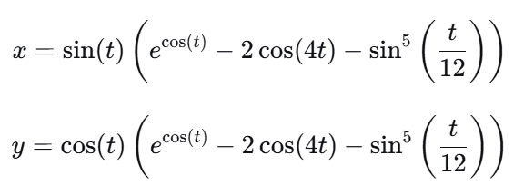
Where the parameter t ranges over the interval  [0,12π].

Figure 1 illustrates the Butterfly Curve.

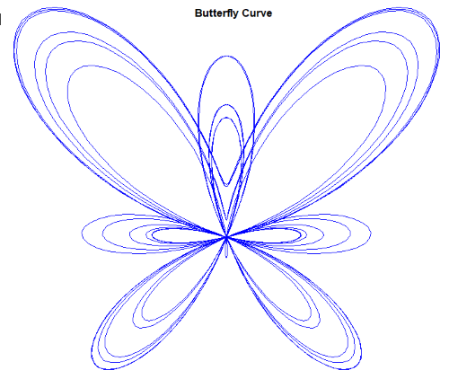
Figure 1: Butterfly Curve

Notably:

• The x-axis values display symmetry, while the y-axis values are asymmetrical.
• The overall structure is nonlinear and cyclical, meaning it repeats its pattern periodically.
• The parametric equation takes a single input (t) and outputs corresponding x and y values.

Code Structure to Construct the Butterfly Curve: 

At this point we show how the butterfly curve was plotted on the chart using script file.

#include <Canvas\Canvas.mqh>

The first step is to include the Canvas library in MQL5 using the line. This library provides all the necessary classes and functions required to draw and visualize the Butterfly Curve on the chart. 

   // Create canvas for drawing
   int width = 800;   // Canvas width
   int height = 600;  // Canvas height
   string canvas_name = "ButterflyCurve";
   
   // Create canvas object
   CCanvas canvas;
   if(!canvas.CreateBitmapLabel(canvas_name, 200, 50, width, height, COLOR_FORMAT_XRGB_NOALPHA))
     {
      Print("Error creating canvas: ", GetLastError());
      return;
     }

First, the canvas dimensions are defined — with a width of 800 pixels and a height of 600 pixels — and the canvas name is set as "ButterflyCurve" . These parameters determine the size and label of the drawing area that will appear on the chart.

Next, a Canvas object (CCanvas canvas) is declared, which serves as the graphical surface for rendering all visual elements, such as lines, shapes, and text. The CreateBitmapLabel() function is then used to instantiate the canvas at a specific position on the chart — in this case, 200 pixels from the left and 50 pixels from the top. The function also specifies the color format (COLOR_FORMAT_XRGB_NOALPHA), which defines how colors and transparency are processed.

Finally, the code includes an error-handling mechanism: if the canvas creation fails, the program prints an error message containing the error code (GetLastError() ) and stops execution. This ensures that subsequent drawing operations are only performed when the canvas is successfully created and ready for use.

   // Set up drawing parameters
   int points = 1000;            // Number of points
   double t_start = 0;           // Start angle
   double t_end = 12 * M_PI;     // End angle
   double step = (t_end - t_start) / (points - 1);
   
   // Calculate curve points
   double x[], y[];
   ArrayResize(x, points);
   ArrayResize(y, points);
   
   for(int i = 0; i < points; i++)
     {
      double t = t_start + i * step;
      double expr = MathExp(MathCos(t)) - 2 * MathCos(4 * t) - MathPow(MathSin(t/12), 5);
      x[i] = MathSin(t) * expr;
      y[i] = MathCos(t) * expr;
     }

This portion of the code defines the mathematical setup and data structure needed to generate the Butterfly Curve before plotting it on the canvas.

First, it establishes the drawing parameters:

• points specifies the number of data points (1000) that will be used to draw the curve, ensuring a smooth and continuous line,
• t_start and t_end define the range of the variable t, which acts as the parameter for the Butterfly Curve equation — here, from 0 to 12π,
• step determines the incremental change in t between each point, ensuring an even distribution of data along the curve.

Next, two dynamic arrays, x[] and y[], are created and resized to hold all the computed coordinates of the Butterfly Curve. Each element in these arrays corresponds to one point on the curve.

Within the for loop, the Butterfly Curve equation is calculated for each value of t. These computed values represent the geometric coordinates of the Butterfly Curve, which are later used for scaling and plotting on the canvas.

   // Find coordinate bounds for scaling
   double x_min = x[ArrayMinimum(x)];
   double x_max = x[ArrayMaximum(x)];
   double y_min = y[ArrayMinimum(y)];
   double y_max = y[ArrayMaximum(y)];
   
   // Scale points to canvas coordinates
   int x_px[], y_px[];
   ArrayResize(x_px, points);
   ArrayResize(y_px, points);
   
   double x_scale = (width - 40) / (x_max - x_min);
   double y_scale = (height - 40) / (y_max - y_min);
   double scale = MathMin(x_scale, y_scale); // Maintain aspect ratio
   
   for(int i = 0; i < points; i++)
     {
      x_px[i] = (int)((x[i] - x_min) * scale) + 20;
      y_px[i] = height - (int)((y[i] - y_min) * scale) - 20; // Flip Y-axis for canvas coordinates
     }

This section of the code handles the scaling and coordinate transformation of the computed Butterfly Curve data points so that they fit neatly within the canvas area.

First, the program determines the coordinate bounds of the curve by finding the minimum and maximum values of both the x and y arrays. These values define the full range of the Butterfly Curve in both directions and are essential for correctly mapping the data to the screen.

Next, two new integer arrays — x_px and y_px — are created and resized to match the number of data points. These arrays will store the pixel-based coordinates that correspond to the scaled version of the curve.

The scaling factors are then computed:

• x_scale converts the range of x-values to the available canvas width (leaving a 20-pixel margin on each side).
• y_scale converts the range of y-values to the available canvas height (also with margins). To ensure that the curve maintains its aspect ratio (so it isn’t stretched or distorted), the smaller of these two scaling factors is selected as the final scale value.

Finally, each data point is transformed into canvas coordinates.

The formula translate the mathematical x–y values into screen positions, taking into account the margins and inverting the Y-axis (since canvas coordinates start from the top-left corner). At the end of this process, all Butterfly Curve data points are properly scaled and positioned within the visible canvas area, ready for plotting.

   // Draw the curve
   canvas.Erase(ColorToARGB(clrWhite, 255)); // White background
   
   // Set line color - we'll pass this directly to Line() method
   uint line_color = ColorToARGB(clrBlue, 255);
   
   // Draw the polyline
   for(int i = 1; i < points; i++)
     {
      canvas.Line(x_px[i-1], y_px[i-1], x_px[i], y_px[i], line_color);
     }
   
   // Title
   canvas.FontSet("Arial", 20, FW_BOLD);
   canvas.TextOut(300, 20, "Butterfly Curve", ColorToARGB(clrBlack, 255));
   
   // Update display
   canvas.Update();

This section of the code focuses on rendering and styling the final Butterfly Curve on the canvas. We configure the plot's visual style by setting the canvas background to white and the data line to blue. The data points from  x_px  and  y_px  are then plotted. Finally, we set the title font to 20-point Arial in black and update the canvas to display the final visualization.

Developing the Butterfly Oscillator

To construct the Butterfly Oscillator, we use the x-component of the butterfly curve because of its symmetrical property. The x-component is naturally bounded within the range [-3, +3], making it ideal for creating an oscillator.

To adapt this for trading, we define the input parameter  t  simply as the elapsed number of price bars. Since t represents bar count, the curve is identical across all timeframes. The underlying equation is cyclical, because of that the oscillator forms wave-like patterns that repeat after each complete cycle.

A complete cycle of the underlying butterfly curve occurs at t=24π, or approximately 75.4 bars. To control the oscillator's sensitivity, we introduce a step size (Δt)as a scaling factor.The number of bars (N) required for a full oscillator cycle is calculated as:  N = 24π / Δt

Examples:

• Step size = 1:     N=24π/1=76 bars (complete cycle)
• Step size = 0.5:  N=24π/0.5=151 bars
• Step size = 5:     N=24π/5=15 bars

The step size directly influences the oscillator’s behavior:

• Smallerstep sizes produce smoother and slower waveforms.
• Largerstep sizes create faster, more frequent oscillations.

This allows traders to customize the oscillator for either long-term pattern detection or short-term cycle analysis.

Making the Oscillator Price-Reactive:

While the oscillator can operate purely based on bar count, it can also be made responsive to price movement. To achieve this, we incorporate the difference between the candle’s closing and opening prices. This adjustment allows the oscillator to react to changes in price dynamics, making it more adaptive to real-time market volatility rather than depending solely on time progression.

This hybrid design—combining cyclical behavior with price sensitivity—enables the Butterfly Oscillator to provide both structural timing and momentum-based confirmation.

Before demonstrating how the oscillator performs in practice, let’s briefly outline the code structure used to implement it. 

//--- plot Butterfly
#property indicator_label1  "Butterfly Oscillator"
#property indicator_type1   DRAW_LINE
#property indicator_color1  DodgerBlue
#property indicator_width1  2
#property indicator_style1  STYLE_SOLID

//--- indicator levels
#property indicator_level1  2.5
#property indicator_level2 -2.5
#property indicator_level3  0.0

This section of the code sets the visual and structural properties of the Butterfly Oscillator. It defines how the indicator appears on the chart — using a solid DodgerBlue line as default, labeled “Butterfly Oscillator,” with a thickness of 2 for clear visibility. Additionally, it establishes key reference levels at 2.5, -2.5, and 0.0. Overall, these settings ensure the oscillator is visually distinct and analytically useful for identifying market cycles.

//--- input parameters
input bool   UsePriceStep = false; // Use ClosePrice as Step size for t increment
input double tmStep       = 0.05;  // Step size for t increment

This section defines user input parameters that control how the Butterfly Oscillator calculates its time increments.

• UsePriceStep: A Boolean option that lets the user choose whether to base the step size on price movement instead of a number of bars.
• tmStep: A numeric input that sets the fixed step size for incrementing the variable t.

These inputs give traders flexibility to adjust how smoothly or sensitively the oscillator responds to market changes. The chosen step size greatly influences the oscillator’s behavior and overall dynamics.

double CalButterflyValue(int bar_index, double bar_close, double bar_open)
  {
   double tStep = UsePriceStep ? MathMod((bar_close - bar_open) / _Point, tmStep) : tmStep;
   double t = bar_index * tStep;

   // Butterfly curve formula
   double x = MathSin(t) *
              (MathExp(MathCos(t)) - 2.0 * MathCos(4.0 * t) - MathPow(MathSin(t / 12.0), 5));

   return (x);
  }

This section defines the Butterfly function, which calculates the oscillator’s value for each bar on the chart.

The function CalButterflyValue() takes three parameters:

• bar_index – the position of the current bar on the chart,
• bar_close – the closing price of that bar, and
• bar_open – the opening price of that bar.

Inside the function, a step size (tStep) is computed. If UsePriceStep is enabled, it dynamically adjusts based on price movement; otherwise, it uses the fixed tmStep value. The variable t is then derived from the bar index and the step size.

Finally, the Butterfly curve formula is applied to compute x, representing the oscillator’s value at that bar. This value captures the mathematical shape of the Butterfly curve and is returned for plotting on the chart.

   int pStart = prev_calculated == 0 ? 0 : prev_calculated - 1;

   for(int i = pStart; i < rates_total; i++)
     {
      double bar_close = close[i];
      double bar_open  = open[i];
      ButterflyBuffer[i] = CalButterflyValue(i, bar_close, bar_open);
     }

This section initializes and fills the Butterfly Oscillator buffer with computed values for chart plotting.

The variable pStart determines where the calculation should begin — starting from zero for the first run, or from the last calculated bar on subsequent updates to improve efficiency. Each calculated value is stored in the ButterflyBuffer array, which is later used to plot the oscillator line in the indicator window.

Demonstrating the Butterfly Oscillator

In our demonstration of the Butterfly Oscillator, we examine its behavior under two conditions: using bar count only and using bar count combined with price action. This comparison allows us to observe how the oscillator responds in each scenario.

Case 1: The Effect of Step Size (Bar Count Only)

Figure 2 illustrates the oscillator when it is driven solely by bar count. In this case, the parameter UsePriceAction is set to false, meaning that only the number of bars determines the oscillator’s progression. Three different step sizes—0.05, 0.5, and 5—are used to study their effects on the waveform.

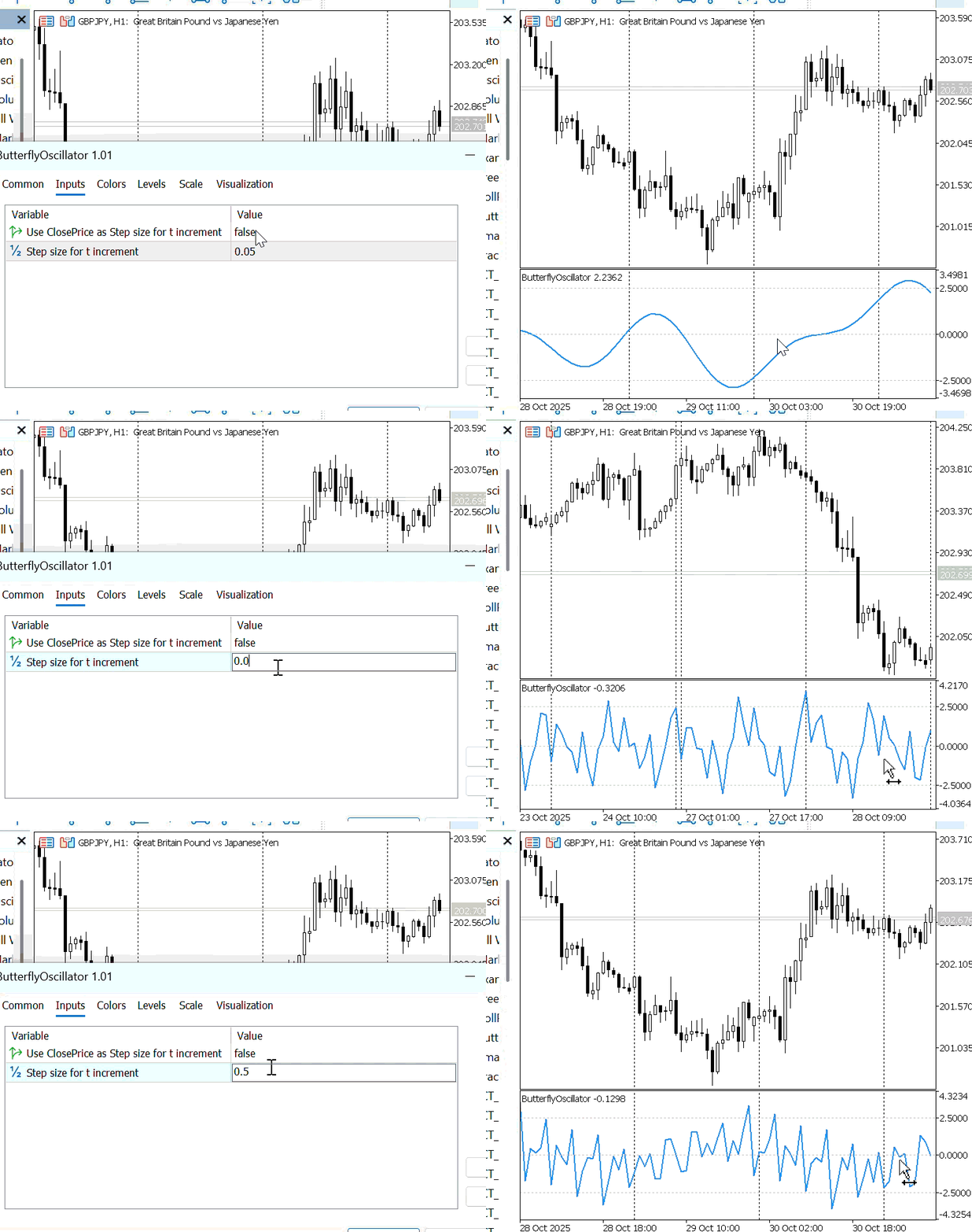
Figure 2: Butterfly Oscillator without Price Action

From the graph, it can be observed that:

• When the step size is small (e.g., 0.05), the oscillator takes longer to complete a full cycle, producing a smoother and more gradual wave.
• When the step size is large (e.g., 5), the oscillator completes its cycle much faster, resulting in a sharper and more irregular pattern.

This demonstrates that the step size directly controls the oscillator’s smoothness and frequency—smaller steps emphasize long-term cyclical movements, while larger steps highlight short-term fluctuations.

Case 2: The Effect of Step Size (With Price Action)

Figure 3 illustrates the oscillator pattern when it is driven by price action. In this case, the oscillator’s behavior is influenced not only by the step size but also by market price movements. Similar to the bar count mode, the oscillator moves faster with larger step sizes and slower with smaller step sizes. However, unlike the previous case, the inclusion of price action adds variability to the curve.

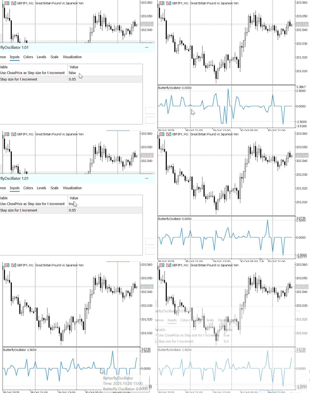
Figure 3: Butterfly Oscillator  Driven by Price Action

Because price action tends to move in a chaotic and nonlinear manner, its fluctuations are reflected in the shape of the oscillator. As a result, the Butterfly Oscillator becomes more dynamic, adapting its waveform to the underlying market volatility rather than following a purely mathematical rhythm.

Butterfly Oscillator Trading Strategy

Now that we have successfully developed the Butterfly Oscillator indicator, we can proceed to build a simple Butterfly Expert Advisor (EA) that uses this indicator as the entry criterion. The trading strategy is designed to detect cyclical turning points in the oscillator and align them with the broader market trend indicated by the Moving Average (MA).

In this approach, we define two strategies for market entry:

Strategy 1

• Buy Signal: When the Moving Average (MA) indicates an uptrendand the Butterfly Oscillator crosses above +2.5, open a buy position
• Sell Signal: When the MA indicates a downtrend and the Butterfly Oscillator crosses above +2.5, open a sell position.

Strategy 2

• Buy Signal: When the MA indicates an uptrend and the Butterfly Oscillator crosses below -2.5, open a buy position.
• Sell Signal: When the MA indicates a downtrend and the Butterfly Oscillator crosses below -2.5, open a sell position.

In both strategies, the MA trend direction serves as the trend filter, while the Butterfly Oscillator acts as the entry trigger.

• Strategy 1 focuses on upper threshold (+2.5) signals, typically identifying the Peak of  oscillator cycles.
• Strategy 2 focuses on lower threshold (-2.5) signals, capturing the trough of the cycle.

The Butterfly EA provides flexibility by allowing traders to choose between Strategy 1 and Strategy 2, or to run both sequentially. The EA also includes an option to determine whether the Butterfly Oscillator should react to price movements or rely solely on bar count progression.

The relevant input parameters are defined as follows:

//--- Strategy Selection
input bool UsePriceStep = false;      // Use ClosePrice 
input bool EnableStrategy1 = true;    // Enable Strategy 1 Peak
input bool EnableStrategy2 = false;   // Enable Strategy 2 Trough

UsePriceStep – Enables or disables the price action mode.

• When set to true, the EA incorporates price movement (close-open difference)into the oscillator’s behavior, making it responsive to market dynamics.
• When set to false, the oscillator relies solely on bar count, maintaining a fixed cyclical pattern.

Strategy Selection:

• Strategy 1 is designed to generate signals based on the peak formations of the oscillator.
• Strategy 2 is designed to generate signals based on its trough formations.

When both Strategy 1 and Strategy 2 are active, the EA gives priority to whichever threshold condition is triggered first during market execution.

To ensure disciplined trade management, the EA is designed to allow only one open position at a time. This prevents conflicting trades from being executed simultaneously, maintaining clarity in strategy performance evaluation.

The core trading logic for the Butterfly EA is implemented as follows:

   //--- Strategy 1: Peak
   if(EnableStrategy1 && prevValue < 2.5 && currValue > 2.5)
   {
      if(maFast > maSlow)
         OpenBuy();
      else if(maFast < maSlow)
         OpenSell();
   }

   //--- Strategy 2: Trough
   if(EnableStrategy2 && prevValue > -2.5 && currValue < -2.5)
   {
      if(maFast > maSlow)
         OpenBuy();
      else if(maFast < maSlow)
         OpenSell();
   }

Strategy 1 (Peak):

When the previous Butterfly Oscillator value is below +2.5 and the current value crosses above +2.5, a signal is generated.

• If the fast MA is above the slow MA, it indicates an uptrend, and a buy order is executed.
• If the fast MAis below the slow MA, it indicates a downtrend, and a sell order is placed.

Strategy 2 (Trough):

When the previous Butterfly Oscillator value is above –2.5 and the current value crosses below –2.5, a signal is generated.

• If the fast MA is above the slow MA, the EA interprets this as an uptrend, and a buy order is executed.
• If the fast MA is below the slow MA, indicating a downtrend, a sell order is issued.

Testing the Butterfly Oscillator EA:

To tailor the EA to individual trading preferences and risk management rules, a comprehensive set of input parameters is provided. These settings are categorized for clarity and allow users to control trade management, indicator behavior, and strategy selection.

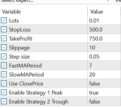
Figure 4: EA Input Parameters

Strategy Testing and Entry Signal Demonstration:

• Step Size : 0.3:

To demonstrate the entry signals generated by the Butterfly EA, we tested Strategy 1 using a step size of 0.3.

Figure 5 illustrates the resulting buy and sell signals produced under this configuration. With a larger step size, the Butterfly Oscillator completes its cycle over fewer bars, allowing it to reach its peaks and troughs more quickly. As a result, the EA generates more frequent entry signals within a shorter time span.

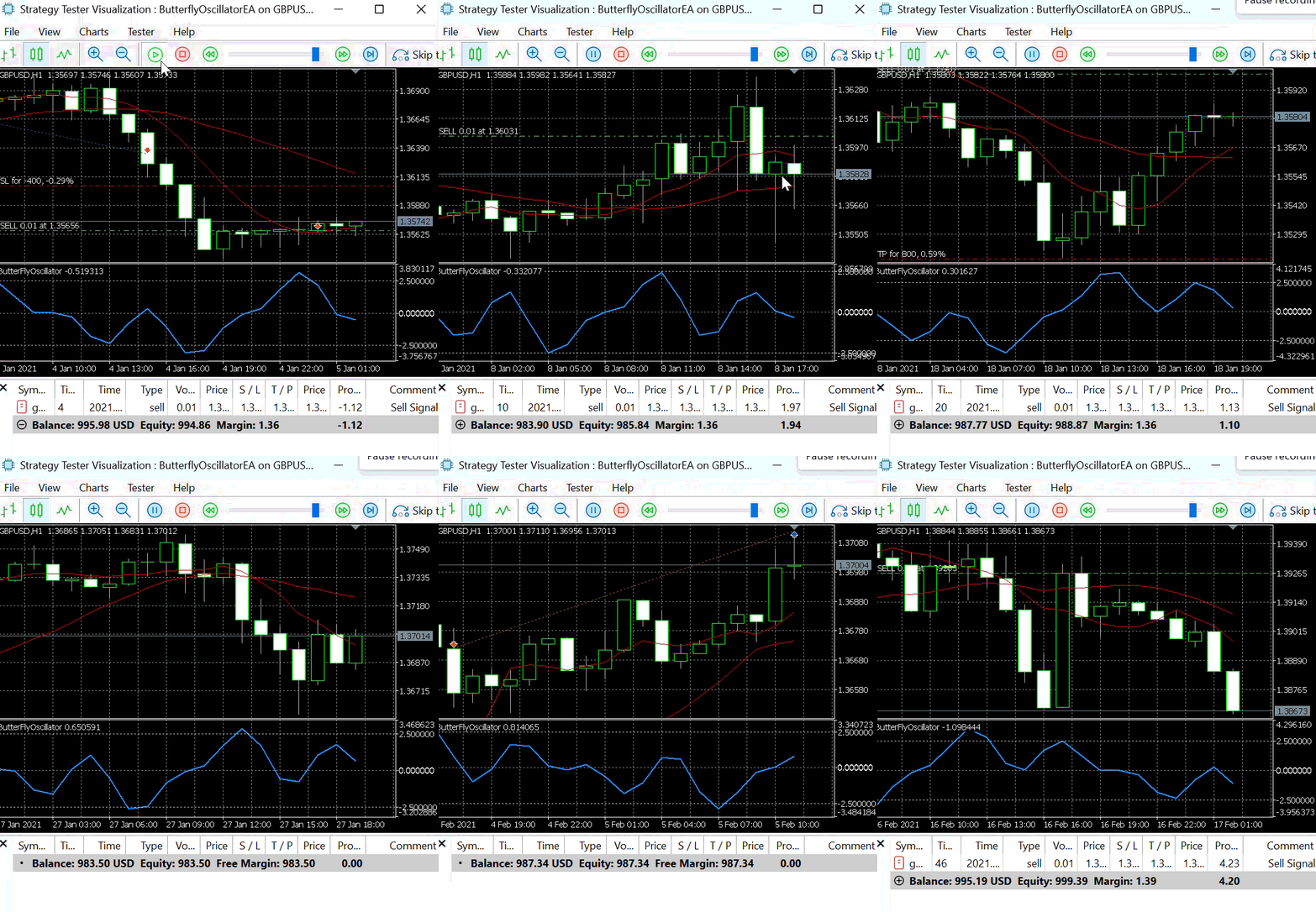
Figure 5: Strategy 1 with Step Size =0.3

• Step Size : 0.03:

Using a step size of 0.03, we further examined the behavior of the Butterfly Expert Advisor under Strategy 1.

Figure 6 presents the buy and sell signals generated with this smaller step size. When the step size is small, the Butterfly Oscillator requires more bars to complete a full cycle. Consequently, it reaches its peaks and troughs more slowly, resulting in fewer entry signals being produced over the same period.

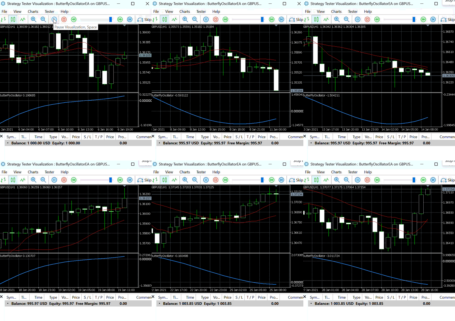
Figure 6: Strategy 1 with Step Size =0.03

This behavior highlights the direct influence of the step size on trading signal frequency—larger values lead to faster oscillations and more trades, while smaller values create slower, smoother cycles with fewer but more stable signals.

Conclusion

In this article, we used the Butterfly Curve concept to build an oscillator and a trading strategy. The Butterfly Oscillator demonstrated how mathematical patterns can be adapted to market dynamics, providing unique insights into price movements. By varying the step size, we observed how the oscillator’s smoothness and signal frequency change, and how these characteristics can influence trade entries when combined with moving average trends.

The developed Butterfly EA successfully applied the oscillator as an entry criterion, offering two distinct strategies—one for peaks and another for troughs—each responsive to both market direction and oscillator thresholds.

In our next article, we will experiment with various instruments to test the strength and weakness of this concept. We will further experiment with this new oscillator in combination with other oscillators to fine-tune our entry strategy. Stay tuned for more entry tips and enhancements to the Butterfly trading system.

File	Description
ButterflyPlot.mq5	This script file is responsible for generating and displaying the Butterfly Curve on the active chart window using its defined mathematical function. When the script is executed, it plots the curve visually on the chart window. Once the Butterfly Curve is drawn, it remains displayed on the chart as part of the current visual layer. The curve generated by this script can only be cleared or removed when the chart’s template is changed or updated to a new one.
ButterflyOscillator.mq5	This file defines the Butterfly Indicator, which is designed to appear in a separate subwindow below the main price chart.
ButterflyOscillatorEA.mq5	This file defines an Expert Advisor that utilizes the Butterfly Oscillator to automatically open and manage trading positions the platform.