Neural Networks in Trading: Unraveling Structural Components (Encoder)

Introduction

We are continuing our work to implement our own vision of the approaches presented by the authors of the SCNN framework. As a reminder, SCNN (Structured Component Neural Network) offers a conceptually different approach: instead of attempting to model the entire time series using a single universal mechanism, it divides it into five key components — long-term, seasonal, short-term, coupled, and residual. Each of these components is modeled and extrapolated separately, which not only gives us flexibility but also allows us to obtain an interpretable result at every stage.

The main advantage of this architecture is transparency. Unlike traditional black boxes, SCNN allows analysts and traders to see exactly which part of the model is responsible for a particular segment of the forecast and how confident the model is under current conditions. This is particularly important when working with financial data, where trust in the model must be supported by explainability and controllability. In addition, a tailored approach to extrapolating each component makes it possible to use both statistical heuristics (for long-term and seasonal patterns) and trainable neural network modules (for modeling short-term anomalies or interdependencies between assets).

The framework also accounts for complex temporal dependencies, including autocorrelation relationships, which are often ignored in simplified models. This is particularly relevant for tasks related to intraday trading or forecasting at the boundary between trading sessions. SCNN allows dynamic adaptation to real-time statistical shifts and also helps identify anomalous points where the forecast may be unreliable.

The author's visualization of the SCNN framework is shown below.

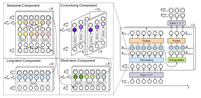
In the practical section of our previous work, we developed the CNeuronPeriodNorm object, designed to extract periodic components from a time series. This component became the first step toward implementing the SCNN framework in the MQL5 environment and will be used to extract long-term and short-term components. The use of OpenCL kernels enables efficient parallel data processing and supports the backpropagation mechanism, making this module suitable for use within trainable neural network architectures.

Later, we will show that, through a few simple data transformations, CNeuronPeriodNorm can also be adapted to extract the seasonal component, which makes it even more versatile. Today, we will take the next step: we will start building an object responsible for extracting the coupled component, which reflects interrelated changes among several variables in a time series. This module will play a key role in modeling synchronized oscillations and anomalous co-movements, which is particularly relevant in the context of multivariate market analysis.

Extraction of the coupled component

Our practical experience shows that a temporal analysis alone is not sufficient for the correct implementation of the model. It is also important to take into account spatial dependencies — that is, the relationships between different variables at any given moment in time. This is precisely what the coupled component extraction mechanism does: it helps detect same-direction or opposite-direction movements between the signals of individual component sequences in the analyzed multimodal time series. Such coevolution can be either stable or dynamically changing, and therefore requires an adaptive approach to normalization.

Within the SCNN framework, this problem is solved by implementing spatially weighted normalization using an attention mechanism. We will now move on to the next implementation step, in which we will present our own interpretation of the proposed algorithm, guided by the practical needs of financial modeling. As usual, we delegate the bulk of the calculations — including weighted averaging and adaptive standardization — to the OpenCL context. This not only speeds up processing but also preserves flexibility in configuring the architecture.

To that end, we will create a new kernel called AdaptSpatialNorm. The kernel algorithm implements adaptive normalization of the input data, taking inter-variable attention into account and thereby ensuring more accurate and sensitive processing of spatial relationships. The idea is to calculate the mean and standard deviation for each time point, weighted by the attention mask. This makes it possible not simply to take an average across all variables, but to account for their relative significance — that is, the influence of each variable on a specific point within a spatiotemporal context.

__kernel void AdaptSpatialNorm(__global const float* inputs,
                               __global const float* attention,
                               __global float2* mean_stdevs,
                               __global float* outputs
                              )
  {
   const size_t i = get_global_id(0);
   const size_t a = get_local_id(1);
   const size_t v = get_global_id(2);
   const size_t total_inputs = get_global_size(0);
   const size_t total_local = get_local_size(1);
   const size_t variables = get_global_size(2);

In the computational kernel, computations are organized across three dimensions: time, variables, and local work-items. Each work-item is responsible for processing a specific value — a single variable at a given point in time. First, an index offset is determined, allowing each work-item to correctly access the required memory regions.

   __local float Temp[LOCAL_ARRAY_SIZE];
   const int shift_v = v * total_inputs;
   const int shift_out = shift_v + i;

Then the main part of the work begins, in which the values from the input array and the corresponding attention weights are retrieved for all variables. Each value is multiplied by its weight, after which local summation is performed — first to calculate the mean, then to determine the variance.

   float mean = 0, stdev = 0;
   for(uint l = 0; l < variables; l += total_local)
     {
      const int shift_at = v * variables + (a + l);
      float val = IsNaNOrInf(inputs[(a + l) * total_inputs + i], 0);
      float att = IsNaNOrInf(attention[shift_at], 0);
      mean += LocalSum(val * att, 1, Temp);
      BarrierLoc;
      stdev += LocalSum(val * val * att, 1, Temp);
      BarrierLoc;
     }

To ensure correct parallel computation across work-items, a synchronization barrier is used, which helps avoid access conflicts when working with shared memory.

Here, it is worth paying special attention to the technical aspects of organizing computations. To correctly perform summation operations on values coming from different work-items, so-called work-groups are created within OpenCL. Work-items within these groups can exchange data via local memory, which, unlike global memory, is significantly faster and allows collective operations such as reduction or summation to be implemented efficiently.

However, this architecture has a natural limitation — the size of the work-group cannot exceed a certain hardware limit set by the graphics card or another computing device. In practice, this means that the number of work-items simultaneously processing variables in a single group is limited and does not always correspond to the dimensionality of the input array being processed.

To work around this limitation, a special loop has been implemented in the kernel body that allows all variables to be iterated over step by step, even if their number significantly exceeds the size of the work-group. The overall feature space is divided into blocks, processed in chunks, and the values are aggregated sequentially. This approach maintains computational efficiency and ensures that all mathematical operations are performed correctly, regardless of the number of variables involved in the model.

This technique makes the implementation robust when scaling and versatile enough to run on a variety of devices with different specifications, while making the model itself more flexible and portable.

Once all values have been processed, only one work-item in each local group takes on the task of final normalization. It calculates the variance by subtracting the square of the mean from the sum of the squares of the values, and then takes the square root to obtain the standard deviation. To prevent division by zero, a safeguard is in place: if the variance is too small, it is replaced with one.

   if(a == 0)
     {
      stdev -= mean * mean;
      stdev = IsNaNOrInf(sqrt(stdev), 1);
      if(stdev <= 0)
         stdev = 1;
      mean_stdevs[shift_out] = (float2)(mean, stdev);
      outputs[shift_out] = IsNaNOrInf((inputs[shift_out] - mean) / stdev, 0);
     }
  }

After that, the normalized input value is calculated and written to the output array. At the same time, the calculated mean and standard deviation are saved — they will be useful later on.

The implemented logic combines the aggregation of information about the spatial distribution of data with normalization based on that distribution. This allows the model to respond sensitively to hidden relationships between variables and, as a result, to capture the dynamics of complex time-series processes more accurately — which is particularly important in financial forecasting.

To fully train the model, it is necessary not only to perform a forward pass that computes normalized values, but also to perform a correct backward pass that ensures the error gradients are propagated back to the input data and parameters. In the context of our AdaptSpatialNorm kernel for spatially weighted normalization, the next logical step is to implement the backward-pass kernel AdaptSpatialNormGrad, which is responsible for distributing the error gradients across the input data and attention weights.

__kernel void AdaptSpatialNormGrad(__global const float* inputs,
                                   __global float* inputs_gr,
                                   __global const float* attention,
                                   __global float* attention_gr,
                                   __global const float2* mean_stdevs,
                                   __global const float2* mean_stdevs_gr,
                                   __global const float* outputs_gr,
                                   const uint total_inputs
                                  )
  {
   const size_t i = get_global_id(0);              // main
   const size_t loc = get_local_id(1);             // local to sum
   const size_t v = get_global_id(2);              // variable
   const size_t total_main = get_global_size(0);   // total
   const size_t total_loc = get_local_size(1);     // local dimension
   const size_t variables = get_global_size(2);    // total variables
//---
   __local float Temp[LOCAL_ARRAY_SIZE];

The algorithm is based on distributing the computational load across work-items, where each work-item processes a specific combination of indices corresponding to a time slice and a variable. Local memory is used to store intermediate values, which speeds up the processes of summing and aggregating data within work-groups.

First, the gradients with respect to the input data are computed. For each element of the input array, the corresponding attention parameters and output gradients are retrieved. Next, the gradient is calculated, taking into account the partial derivatives with respect to the normalization parameters (mean and standard deviation), which also play a role in backpropagation. All partial sums are accumulated, and the result is then stored in the input gradient array.

//--- Input gradient
     {
      if(i < total_inputs)
        {
         float grad = 0;
         int shift_in = v * total_inputs + i;
         float x = IsNaNOrInf(inputs[shift_in], 0);
         for(int l = 0; l < variables; l += total_loc)
           {
            if((l + loc) >= variables)
               break;
            int shift_out = i + (l + loc) * total_inputs;
            float att = IsNaNOrInf(attention[(l + loc) * variables + v], 0);
            float out_gr = IsNaNOrInf(outputs_gr[shift_out], 0);
            float2 ms = mean_stdevs[shift_out];
            float2 ms_gr = mean_stdevs_gr[shift_out];
            float dy = (1 - att) * (1 / ms.y - (x - ms.x) * att * x / pow(ms.y, 3.0f));
            float dmean = IsNaNOrInf(ms_gr.x * att, 0);
            float dstd = IsNaNOrInf(ms_gr.y * x * (att - att * att) / ms.y, 0);
            grad += IsNaNOrInf(dy * out_gr + dmean + dstd, 0);
           }
         grad = LocalSum(grad, 1, Temp);
         if(loc == 0)
            inputs_gr[shift_in] = grad;
        }
      BarrierLoc;
     }

Looking ahead a bit, it is worth noting an important detail: the normalization parameters we have saved (the mean and standard deviation) are not byproducts of the calculations. On the contrary, they actively participate in the subsequent operations of the SCNN framework, forming a kind of auxiliary data processing branch. Therefore, the error gradient accumulated for these parameters during later stages of the forward pass must also be propagated back down to the level of the input data.

This means that during the backward pass, we do not limit ourselves to the main information flow — we also take into account the contribution associated with the derivatives with respect to the stored normalization statistics and add it to the final input gradient. This approach ensures the integrity of the computational graph and allows the model to effectively adjust all parameters that affect the result, including those indirectly related to the input through normalization mechanisms.

Next, the gradients with respect to the attention parameters are computed. For each element of the attention weights, the algorithm iterates through all corresponding time points, using the values from the input data and the output gradients that have already been computed. The calculations also account for the effect of attention on normalization through the mean and standard deviation. The final values are accumulated using local memory and stored in the corresponding attention gradient array.

//--- Attention gradient
     {
      if(i < variables)
        {
         float grad = 0;
         int shift_att = v * variables + i;
         float att = IsNaNOrInf(attention[shift_att], 0);
         for(int l = 0; l < total_inputs; l += total_loc)
           {
            if((l + loc) >= total_inputs)
               break;
            int shift_out = (l + loc) + v * total_inputs;
            int shift_in = (l + loc) + i * total_inputs;
            float x = IsNaNOrInf(inputs[shift_in], 0);
            float out_gr = IsNaNOrInf(outputs_gr[shift_out], 0);
            float2 ms = mean_stdevs[shift_out];
            float2 ms_gr = mean_stdevs_gr[shift_out];
            float dy = -x / ms.y - (x - ms.x) * x * x * (1 - 2 * att) / (2 * pow(ms.y, 3.0f));
            float dmean = IsNaNOrInf(ms_gr.x * x, 0);
            float dstd = IsNaNOrInf(ms_gr.y * x * x * (1 - 2 * att) / (2 * ms.y), 0);
            grad += IsNaNOrInf(dy * out_gr + dmean + dstd, 0);
           }
         grad = LocalSum(grad, 1, Temp);
         if(loc == 0)
            attention_gr[shift_att] = grad;
        }
     }
  }

It is important to note that the implementation accounts for the possibility of invalid numerical values, such as NaN or infinity, and prevents them from propagating, which improves the algorithm's robustness.

This overall approach, with loop-based data processing and the use of local memory, ensures scalability and efficiency, allowing large sets of variables and time steps to be processed even when their size exceeds the work-group dimensions.

Thus, the AdaptSpatialNormGrad kernel enables accurate and efficient calculation of gradients for key normalization parameters while accounting for spatial attention weights, allowing this mechanism to be integrated into complex models trained via backpropagation.

To integrate the spatially weighted normalization algorithm described above into the overall architecture, a specialized CNeuronAdaptSpatialNorm object is created in the main program. This class inherits the base interfaces from CNeuronBaseOCL, which allows it to integrate seamlessly into the hierarchy of neural components. The main purpose of the object is to properly organize the computations for both the forward and backward passes, as well as to correctly process all auxiliary components related to the attention mechanism.

The structure of the new class is shown below.

class CNeuronAdaptSpatialNorm :  public CNeuronBaseOCL
  {
protected:
   uint                    iVariables;
   uint                    iCount;
   //---
   CParams                 cEn;
   CNeuronTransposeOCL     cEnT;
   CNeuronBaseOCL          cEnEnT;
   CNeuronSoftMaxOCL       cAttan;
   CNeuronBaseOCL          cMeanSTDevs;
   //---
   virtual bool      AdaptSpatialNorm(CNeuronBaseOCL *NeuronOCL);
   virtual bool      AdaptSpatialNormGrad(CNeuronBaseOCL *NeuronOCL);
   //---
   virtual bool      feedForward(CNeuronBaseOCL *NeuronOCL) override;
   virtual bool      updateInputWeights(CNeuronBaseOCL *NeuronOCL) override;
   virtual bool      calcInputGradients(CNeuronBaseOCL *NeuronOCL) override;

public:
                     CNeuronAdaptSpatialNorm(void) : iCount(0), iVariables(1) {};
                    ~CNeuronAdaptSpatialNorm(void) {};
   //---
   virtual bool      Init(uint numOutputs, uint myIndex, COpenCLMy *open_cl,
                          uint units_count, uint variables,
                          ENUM_OPTIMIZATION optimization_type, uint batch);
   //---
   virtual bool      Save(const int file_handle) override;
   virtual bool      Load(const int file_handle) override;
   //---
   virtual int       Type(void) override const  {  return defNeuronAdaptSpatialNorm; }
   virtual void      SetOpenCL(COpenCLMy *obj) override;
   //---
   CNeuronBaseOCL*   GetMeanSTDevs(void) { return cMeanSTDevs.AsObject(); }
   virtual uint      GetVariables(void) const { return iVariables; }
   virtual uint      GetUnits(void) const { return iCount; }
   //---
   virtual bool      WeightsUpdate(CNeuronBaseOCL *source, float tau);
  };

Inside the class, we see a number of protected members, each of which plays an important role in the component's operation. The variables iVariables and iCount specify the dimensions of the input data tensor and define the spatial boundaries of processing. The internal objects cEn, cEnT, cEnEnT, and cAttan sequentially form and train the attention matrix. The cMeanSTDevs component completes this chain by storing and updating the normalization parameters used to scale the input data based on the calculated attention weights.

All internal objects are declared statically, which greatly simplifies memory management and initialization. As a result, the solution becomes more reliable and predictable in its behavior: there is no need to manually allocate or release resources. The class constructor and destructor remain empty, since the objects already exist when an instance of the class is created and are automatically destroyed when the instance's life cycle ends.

All of the class's internal components are initialized centrally in the Init method. This method takes key parameters as input that make it possible to uniquely determine the architecture of the object being created, including the dimensionality of the input data. The entire process unfolds in a sequential and logical manner, with a clear connection to the model's internal structure.

bool CNeuronAdaptSpatialNorm::Init(uint numOutputs, uint myIndex, COpenCLMy *open_cl,
                                   uint units_count, uint variables,
                                   ENUM_OPTIMIZATION optimization_type, uint batch)
  {
   if(!CNeuronBaseOCL::Init(numOutputs, myIndex, open_cl, units_count * variables, optimization_type, batch))
      return false;

At the first stage, the method of the same name from the parent class CNeuronBaseOCL is called, which performs the initial setup of the neural node. The size of the results buffer is calculated as the product of the number of variables and the length of the sequence. If the base-level initialization is successful, the parameters of the input data tensor are set and stored in the local variables iVariables and iCount.

   iVariables = variables;
   iCount = units_count;
//---
   uint dimension = (iVariables + 1) / 2;
   uint index = 0;
   if(!cEn.Init(0, index, OpenCL, iVariables * dimension, optimization, iBatch))
      return false;
   cEn.SetActivationFunction(None);

Next, the internal components responsible for forming the attention matrix are configured sequentially. The cEn object is initialized first. It is a tensor of trainable parameters. Its dimensionality is defined as the product of the number of variables and half that number. This dimensionality reduction makes it possible to identify the most significant features for further processing. The activation function is explicitly disabled here, since at this stage a pure linear transformation is required without distorting the output signal.

Next, the transposition object cEnT is initialized, which makes it possible to obtain a transposed copy of the tensor of trainable parameters.

   index++;
   if(!cEnT.Init(0, index, OpenCL, iVariables, dimension, optimization, iBatch))
      return false;
   cEnT.SetActivationFunction(None);
   index++;
   if(!cEnEnT.Init(0, index, OpenCL, iVariables * iVariables, optimization, iBatch))
      return false;
   cEnEnT.SetActivationFunction(None);

The cEnEnT object plays a key role in building the attention mechanism within the SCNN framework. It is designed to store the results of matrix multiplication of the tensor of trainable parameters by its transposed copy. This operation forms a symmetric matrix that reflects the interdependencies and the strength of the correlation between variables within a single time step. The resulting structure makes it possible to explicitly identify which of the analyzed features have the greatest influence on one another.

The cAttan object completes the construction of the attention mechanism. It takes a correlation matrix as input and applies SoftMax normalization to it, distributing attention across the variables. The number of attention heads corresponds to the number of rows in the correlation matrix, which allows for flexible adaptation to the data structure.

   index++;
   if(!cAttan.Init(0, index, OpenCL, iVariables * iVariables, optimization, iBatch))
      return false;
   cAttan.SetHeads(iVariables);

Finally, the cMeanSTDevs object is configured to store pairs of values: the mean and standard deviation calculated using spatially weighted normalization. The dimensionality of this object is twice the number of output neurons, since two parameters must be stored for each element of the results.

   index++;
   if(!cMeanSTDevs.Init(0, index, OpenCL, 2 * Neurons(), optimization, iBatch))
      return false;
   cMeanSTDevs.SetActivationFunction(None);
//---
   return true;
  }

Thus, the Init method creates and configures all the components necessary for the proper functioning of the spatially weighted normalization mechanism within SCNN. The code structure reflects the rigor and modularity of the architecture, in which each block has a clearly defined purpose and interacts with the others in a specified sequence.

After successfully initializing all internal components, we move on to building the forward pass mechanism implemented in the feedForward method. This marks the beginning of a key stage in the layer’s operation, during which the attention matrix is formed and spatially weighted normalization of the input data is performed.

bool CNeuronAdaptSpatialNorm::feedForward(CNeuronBaseOCL *NeuronOCL)
  {
   if(bTrain)
     {
      if(!cEn.FeedForward())
         return false;
      if(!cEnT.FeedForward(cEn.AsObject()))
         return false;
      if(!MatMul(cEn.getOutput(), cEnT.getOutput(), cEnEnT.getOutput(),
                 iVariables, cEnT.GetWindow(), iVariables, 1, false))
         return false;
      if(!cAttan.FeedForward(cEnEnT.AsObject()))
         return false;
     }
//---
   return AdaptSpatialNorm(NeuronOCL);
  }

It is worth emphasizing an important architectural point here: the attention parameters are formed exclusively during training. This is done intentionally, since the attention matrix itself is a static component of the model — it does not adapt to specific input data during operation. In other words, we train universal weights that reflect stable relationships between variables within the time series. This approach ensures stable model behavior on new data, and attention computation can be skipped during inference, significantly speeding up operation without compromising normalization quality.

Next in the forward pass sequence, the AdaptSpatialNorm method is called, serving as a wrapper for the kernel of the same name. This is the step that transfers control to the OpenCL context, where the main computations take place: normalizing the input data based on the attention weights.

It is worth saying a few words about how the wrapper method for the OpenCL kernel is organized. Although the overall logic of the algorithm remained the same, structural improvements were made to the implementation to enhance the code's readability and reliability. This primarily applies to the way calls to OpenCL functions are written.

Substitution macros were introduced to simplify and standardize the setting of kernel arguments and launching the kernel. For example, the setBuffer macro wraps a call to OpenCL.SetArgumentBuffer with automatic error handling and debug output, including the kernel name, error code, and the line where the failure occurred. The setArgument macro works similarly for setting scalar values.

#define setBuffer(kernel, id, buffer)  if(!OpenCL.SetArgumentBuffer(kernel, id, buffer)) { \
                                          printf("Error of set parameter kernel %s: %d; line %d",
                                                 OpenCL.GetKernelName(kernel), GetLastError(), __LINE__); \
                                          return false; }
#define setArgument(kernel, id, value) if(!OpenCL.SetArgument(kernel, id, value)) { \
                                          printf("Error of set parameter kernel %s: %d; line %d",
                                                 OpenCL.GetKernelName(kernel), GetLastError(), __LINE__); \
                                          return false; }

The kernel is launched using the kernelExecute and kernelExecuteLoc macros, which hide all the technical boilerplate involved in initializing the work-item grid and, on failure, automatically display a detailed textual description of the error linked to the name of the invoked function.

#define kernelExecute(kernel,offset,global)  if(!OpenCL.Execute(kernel, global.Size(), offset, global)) { \
                                                string error; \
                                                CLGetInfoString(OpenCL.GetContext(), CL_ERROR_DESCRIPTION, error); \
                                                printf("Error of execution kernel %s %s: %s", __FUNCSIG__,
                                                        OpenCL.GetKernelName(kernel), error); \
                                                return false; }
#define kernelExecuteLoc(kernel,offset,global,local)  if(!OpenCL.Execute(kernel, global.Size(), offset,
                                                                         global, local)) {  string error; \
                                                         CLGetInfoString(OpenCL.GetContext(), CL_ERROR_DESCRIPTION,
                                                                                                          error); \
                                                         printf("Error of execution kernel %s %s: %s", __FUNCSIG__,
                                                                 OpenCL.GetKernelName(kernel), error); \
                                                         return false; }

Thanks to this structure, the method's code becomes more compact, logically clearer, and easier to scale when new kernels or parameters are added.

In addition, as already mentioned in the description of kernels, before running them, it is necessary to take into account the technical limitations of the computing device — in particular, the maximum size of the work-group supported by the OpenCL platform. These parameters vary depending on the graphics adapter model and can significantly affect the correct execution of the code.

In the body of the AdaptSpatialNorm method, this is implemented by calling CLGetDeviceInfo, which is used to query the valid work-group size for each dimension. The returned values are stored in the union sizes structure, which makes it convenient to access them as an array of integers without having to worry about the specifics of the internal data representation.

bool CNeuronAdaptSpatialNorm::AdaptSpatialNorm(CNeuronBaseOCL *NeuronOCL)
  {
   if(!OpenCL || !NeuronOCL)
      return false;
   uint global_work_offset[3] = { 0 };
   union sizes
     {
      long data[3];
      uchar cdata[24];
     } max_workgroup_size;
   uint size = 0;
   if(!CLGetDeviceInfo(OpenCL.GetContext(), CL_DEVICE_MAX_WORK_ITEM_SIZES, max_workgroup_size.cdata, size))
      return false;

After obtaining these parameters, we form the global_work_size array, which defines the overall computation grid. Moreover, for the second dimension, which determines the width of the local work-group, we explicitly limit the value to the minimum between the number of variables, iVariables, and the maximum size allowed by the device. This ensures that the loop implemented in the kernel will execute correctly even with large volumes of data.

   uint global_work_size[] = { iCount, MathMin(iVariables, uint(max_workgroup_size.data[1])), iVariables};
   uint local_work_size[] = { 1, global_work_size[1], 1};
//---
   uint kernel = def_k_AdaptSpatialNorm;
   setBuffer(kernel, def_k_asn_inputs, NeuronOCL.getOutputIndex())
   setBuffer(kernel, def_k_asn_mean_stdevs, cMeanSTDevs.getOutputIndex())
   setBuffer(kernel, def_k_asn_attention, cAttan.getOutputIndex())
   setBuffer(kernel, def_k_asn_outputs, getOutputIndex())
   kernelExecuteLoc(kernel, global_work_offset, global_work_size, local_work_size)
//---
   return true;
  }

At the same time, the local_work_size array is created, with the number of work-items along the second dimension fixed explicitly. This approach allows for the efficient use of local memory when processing feature vectors.

Next, we sequentially set the kernel argument buffers using the previously defined setBuffer macros, which ensures consistent and safe initialization of the parameters. The process concludes with the kernelExecuteLoc macro, which launches the AdaptSpatialNorm kernel while taking into account all previously specified constraints and the computational grid structure.

In this way, we implement not only a wrapper for calling the kernel, but also a flexible mechanism for adapting the algorithm to the specific technical capabilities of the target hardware, ensuring compatibility and stable operation across a wide range of devices.

The next important step is the distribution of the error gradient, implemented in the calcInputGradients method. This is where the signal propagates backward through the internal objects. The accumulated errors are progressively transformed, propagating back to the trainable parameters of the input level. This part of the algorithm is particularly important because it allows the weights to be updated based on current information about the discrepancy between the predicted and actual values.

bool CNeuronAdaptSpatialNorm::calcInputGradients(CNeuronBaseOCL *NeuronOCL)
  {
   if(!AdaptSpatialNormGrad(NeuronOCL))
      return false;

The process begins by calling the AdaptSpatialNormGrad method, which, like its forward pass counterpart, is a wrapper for the corresponding OpenCL kernel. It is responsible for propagating the gradient from the outputs of the normalization block downward to the input data and the trainable parameters of the attention matrix.

The implementation of the AdaptSpatialNormGrad method almost entirely follows the structure previously used to enqueue the forward pass kernel. We also define the global and local work sizes, set up the buffers using macros, and pass the parameters to the kernel in the correct order. However, there is an important distinction here that stems from the very nature of backpropagating the error.

Whereas during the forward pass each element was processed independently, the situation changes when computing gradients: for each element at the input data level, the gradient contribution from all univariate sequences must be aggregated via attention weights. This requires simultaneous access to many different components of the output tensor, which means a more complex summation scheme.

A special approach is also required for the attention weights. Here, it is necessary to carefully integrate the gradient over the time dimension — that is, to collect information across all positions in the sequence where the corresponding weight was applied. This is a fairly resource-intensive operation, especially when dealing with large input tensors, so special attention is paid to the size of the work-group.

Consequently, for correct and efficient problem setup, the work-group size is chosen as the maximum over the axes along which gradients need to be aggregated, while also accounting for the maximum permissible value supported by a specific OpenCL device. This approach not only ensures compliance with technical requirements but also optimizes performance by avoiding unnecessary overflows and memory access conflicts.

After computations on the OpenCL side are complete, the method continues in a more familiar style. We successively propagate the error gradient down through the objects that form the attention matrix.

   if(!cEnEnT.CalcHiddenGradients(cAttan.AsObject()))
      return false;
   if(!MatMulGrad(cEn.getOutput(), cEn.getPrevOutput(),
                  cEnT.getOutput(), cEnT.getGradient(),
                  cEnEnT.getGradient(), iVariables,
                  cEnT.GetWindow(), iVariables, 1, false))
      return false;
   if(!cEn.CalcHiddenGradients(cEnT.AsObject()) ||
      !SumAndNormilize(cEn.getGradient(), cEn.getPrevOutput(), cEn.getGradient(),
                       cEnT.GetWindow(), false, 0, 0, 0, 1))
      return false;
   if(cEn.Activation() != None)
      if(!DeActivation(cEn.getOutput(), cEn.getGradient(), cEn.getGradient(), cEn.Activation()))
         return false;
//---
   return true;
  }

Thus, the entire calcInputGradients method is a clearly structured sequence of steps that ensures the error is propagated backward through the network consistently and correctly.

The parameter optimization method is implemented here as concisely as possible, yet with a very clear purpose. The entire task comes down to passing control to a single internal object, cEn, which contains the trainable attention parameters. This object represents the core of the parametric block on which the correlation matrix is built. It alone bears full responsibility for the trainable part of the module.

bool CNeuronAdaptSpatialNorm::updateInputWeights(CNeuronBaseOCL *NeuronOCL)
  {
   return cEn.UpdateInputWeights();
  }

The complete code of the CNeuronAdaptSpatialNorm class and all its methods is provided in the attachment for further study.

SCNN Encoder

After we have built the objects responsible for extracting individual components of the time series, the next logical step is to integrate them into a single coherent structure: the SCNN Encoder. At this stage, the pre-formed blocks are assembled into a clearly defined sequence that ensures reliable, stable, and yet flexible processing of the data being analyzed.

The key feature of the SCNN Encoder is its modular architecture. It is based on four parallel branches, each responsible for its own scale of analysis. One captures long-term trends, another captures seasonal patterns, a third captures short-term fluctuations, and the fourth adaptively normalizes the data, enhancing the relationships between individual features.

All of these algorithms are carefully implemented within the specialized CNeuronSCNNEncoder object. Its structure embodies the described logic and lays the foundation for forming a generalized representation of the sequence — compressed, meaningful, and suitable for further forecasting.

class CNeuronSCNNEncoder   :  public CNeuronTransposeOCL
  {
protected:
   CNeuronPeriodNorm       cLongNorm;
   CNeuronTransposeVRCOCL  cSeasonTransp;
   CNeuronPeriodNorm       cSeasonNorm;
   CNeuronTransposeVRCOCL  cUnSeasonTransp;
   CNeuronPeriodNorm       cShortNorm;
   CNeuronAdaptSpatialNorm cAdaptSpatNorm;
   CNeuronBaseOCL          cConcatenated;
   CNeuronSwiGLUOCL        cProjection;
   CNeuronTransposeOCL     cTranspose;
   CNeuronConvOCL          caFusion[2];
   CNeuronBaseOCL          cFusionOut;
   //---
   virtual bool      feedForward(CNeuronBaseOCL *NeuronOCL) override;
   virtual bool      updateInputWeights(CNeuronBaseOCL *NeuronOCL)  override;
   virtual bool      calcInputGradients(CNeuronBaseOCL *NeuronOCL)  override;

public:
                     CNeuronSCNNEncoder(void) {};
                    ~CNeuronSCNNEncoder(void) {};
   //---
   virtual bool      Init(uint numOutputs, uint myIndex, COpenCLMy *open_cl,
                          uint units_count, uint variables, uint forecast,
                          uint season_period, uint short_period,
                          ENUM_OPTIMIZATION optimization_type, uint batch);
   //---
   virtual bool      Save(const int file_handle) override;
   virtual bool      Load(const int file_handle) override;
   //---
   virtual int       Type(void) override const  {  return defNeuronGinAR; }
   virtual void      TrainMode(bool flag) override;
   virtual void      SetOpenCL(COpenCLMy *obj);
   //---
   virtual bool      WeightsUpdate(CNeuronBaseOCL *source, float tau);
  };

The structure of the new class contains a number of internal objects, each performing a strictly defined function within the Encoder. We'll learn about their purposes a little later, as we explore the logic of the algorithm. At this point, it is worth highlighting an important architectural detail: all of these components are declared statically. This means that memory is allocated for them in advance, and their lifecycle strictly corresponds to the lifecycle of the CNeuronSCNNEncoder object itself. This approach eliminates the need for extra processing — the class constructor and destructor remain empty.

Initialization of all declared and inherited internal objects is implemented in the Init method, whose parameters provide all the constants that define the object's architecture.

bool CNeuronSCNNEncoder::Init(uint numOutputs, uint myIndex, COpenCLMy *open_cl,
                              uint units_count, uint variables, uint forecast,
                              uint season_period, uint short_period,
                              ENUM_OPTIMIZATION optimization_type, uint batch)
  {
   if(!CNeuronTransposeOCL::Init(numOutputs, myIndex, open_cl, units_count + forecast, variables,
                                                                       optimization_type, batch))
      return false;
   SetActivationFunction(None);

It all begins with a call to the base method of the same name in the parent class, where the key parameters of the architecture are specified. After successful initialization, a neutral activation function is enabled, preventing nonlinear distortions from being introduced at this stage.

Next, modules responsible for preprocessing the time series are created one after another. First, the normalization block for the long-term component is initialized.

   uint index = 0;
   if(!cLongNorm.Init(0, index, OpenCL, 1, units_count, variables, optimization, iBatch))
      return false;
   cLongNorm.SetActivationFunction(None);

The next important step is to isolate the seasonal component. In the original concept proposed by the authors of the SCNN framework, this step is interpreted as normalizing the data with a step corresponding to the seasonal period. At first glance, it might seem that this requires some kind of specialized module. However, we approached the problem more rationally, in the spirit of the classical principles of systems engineering.

We developed a universal normalization object designed to process data over fixed periods. On its own, it contains no information about the seasonal structure; that structure appears as soon as we change the representation of the array being analyzed. Simply transposing the sequence of time steps by the length of the seasonal period automatically groups the data into sequences with the required interval. These newly formed sequences are perfectly suited to the format expected by our period-normalization module.

Thus, with minimal effort, we obtain a powerful mechanism for extracting the seasonal component without making any additional changes to the structure of the normalizing object itself. All it takes is to properly reorganize the input data, and from there, a proven and well-tuned algorithm takes over.

   index++;
   if(!cSeasonTransp.Init(0, index, OpenCL, variables, units_count / season_period, season_period,
                                                                            optimization, iBatch))
      return false;
   cSeasonTransp.SetActivationFunction(None);
   index++;
   if(!cSeasonNorm.Init(0, index, OpenCL, cSeasonTransp.GetCount(), season_period, variables,
                                                                       optimization, iBatch))
      return false;
   cSeasonNorm.SetActivationFunction(None);
   index++;
   if(!cUnSeasonTransp.Init(0, index, OpenCL, variables, season_period, cSeasonTransp.GetCount(),
                                                                           optimization, iBatch))
      return false;
   index++;

After isolating the seasonal component, we return the data to its original representation by performing a reverse transposition and activate the short-term normalization block.

   if(!cShortNorm.Init(0, index, OpenCL, units_count / short_period, short_period, variables, optimization, iBatch))
      return false;
   cSeasonNorm.SetActivationFunction(None);
   index++;
   if(!cAdaptSpatNorm.Init(0, index, OpenCL, units_count, variables, optimization, iBatch))
      return false;
   cAdaptSpatNorm.SetActivationFunction(None);

Next comes adaptive spatial normalization, which takes into account the relationships between the variables in the input sequence.

Once the data from various sources have been prepared, a merging module is created to accumulate the outputs of all normalization blocks into a single feature matrix. The size of this module is calculated dynamically, taking into account both the main outputs and the statistical values associated with each normalization block.

   index++;
   uint concatSize = units_count * variables;                                         //inputs
   concatSize += cLongNorm.Neurons() + cLongNorm.GetMeanSTDevs().Neurons();           // long term
   concatSize += cSeasonNorm.Neurons() + cSeasonNorm.GetMeanSTDevs().Neurons();       // seasons
   concatSize += cShortNorm.Neurons() + cShortNorm.GetMeanSTDevs().Neurons();         // short term
   concatSize += cAdaptSpatNorm.Neurons() + cAdaptSpatNorm.GetMeanSTDevs().Neurons(); // spatial
   if(!cConcatenated.Init(0, index, OpenCL, concatSize, optimization, iBatch))
      return false;
   cConcatenated.SetActivationFunction(None);

The next logical component is the projection block, which enables effective compression and restructuring of the multidimensional feature space.

   index++;
   if(!cProjection.Init(0, index, OpenCL, concatSize / variables, concatSize / variables, 
                             units_count + forecast, 1, variables, optimization, iBatch))
      return false;

Its output is sent to a transposition module, which converts data between time and feature representations, depending on the requirements of subsequent processing.

   index++;
   if(!cTranspose.Init(0, index, OpenCL, variables, units_count + forecast, optimization, iBatch))
      return false;
   index++;
   if(!caFusion[0].Init(0, index, OpenCL, variables, variables, variables, units_count + forecast,
                                                                            optimization, iBatch))
      return false;
   caFusion[0].SetActivationFunction(TANH);
   index++;
   if(!caFusion[1].Init(0, index, OpenCL, variables, variables, variables, units_count + forecast,
                                                                            optimization, iBatch))
      return false;
   caFusion[1].SetActivationFunction(SIGMOID);
   index++;
   if(!cFusionOut.Init(0, index, OpenCL, caFusion[0].Neurons(), optimization, iBatch))
      return false;
//---
   return true;
  }

The final stage consists of two parallel convolutional layers that implement different signal filtering mechanisms. One of them uses the hyperbolic tangent function, giving the output a smooth saturation, while the other uses a sigmoid function, providing a logistic bound on the values. Their results converge in the final convolution module, which completes the construction of the architecture.

We've done a great deal of work, and the article has grown considerably in length. Ahead of us is an examination of the nontrivial algorithm for the forward and backward passes of our Encoder — a stage that requires special attention and focus. Therefore, it makes sense to take a short break to give yourself time to absorb and reflect on the material that has already been covered. In the next article, we will continue our work, bring it to its logical conclusion, and evaluate the effectiveness of the implemented solutions using real historical data.

Conclusion

In this article, we examined in detail the next stage in the implementation of the SCNN framework — the construction and integration of the adaptive spatial normalization object, as well as the combination of the main components into a single Encoder. We have demonstrated how a well-designed architecture and the use of modern OpenCL computing technologies make it possible to effectively identify structural components in time series and ensure high-quality data preparation for further forecasting.

In the next article, we will continue our research by focusing on testing and evaluating the performance of the SCNN framework on real-world data, which will allow us to assess the practical significance of the implemented methods and their effectiveness in financial forecasting tasks.

Links

• Disentangling Structured Components: Towards Adaptive, Interpretable and Scalable Time Series Forecasting
• Other articles in the series

Software used in this article

#	Name	Type	Description
1	Study.mq5	Expert Advisor	Expert Advisor for offline model training
2	StudyOnline.mq5	Expert Advisor	Expert Advisor for online model training
3	Test.mq5	Expert Advisor	Expert Advisor for model testing
4	Trajectory.mqh	Class library	Structure for describing the system state and model architecture
5	NeuroNet.mqh	Class library	Class library for building neural networks
6	NeuroNet.cl	Library	Code library for an OpenCL program