Beyond the Mean and Standard Deviation: A Robust Statistics Library for MQL5 Indicators

Contents

1. Introduction
2. Why the classical tools are fragile
3. The shared library: median, MAD, and Theil-Sen
4. Three drop-in indicators
5. Seeing the difference: the comparison overlay
6. The evidence: the breakdown point
7. Edge cases and pitfalls
8. Conclusion

Introduction

Almost every statistical indicator on a MetaTrader chart is built from two numbers: the arithmetic mean and the standard deviation. Bollinger Bands center on a moving average and size themselves with a standard deviation. A linear regression channel fits a least-squares line and widens it by the standard deviation of the residuals. A z-score or sigma oscillator measures how many standard deviations the latest price sits from its mean. These tools are everywhere because the mean and the standard deviation are cheap to compute and easy to reason about, and because they are exactly right when the data is well behaved.

The trouble is that price data is not well behaved. A single bad tick, a weekend gap, a news spike, a stop run, or a thin-liquidity print injects an outlier that the mean and the standard deviation have no defense against. The mean is pulled toward the outlier, the standard deviation balloons, and every band, channel, and oscillator built on them distorts for the entire length of their window. The indicator you were relying on to describe "normal" price behavior is, at the worst possible moment, describing the outlier instead.

This article builds the fix from robust statistics, the branch of statistics designed for exactly this situation: a small library and three drop-in indicators that use it. In place of the mean we use the median; in place of the standard deviation we use the median absolute deviation (MAD); and in place of the least-squares slope we use the Theil-Sen slope, the median of all pairwise slopes. Each of these has a property the classical estimator lacks, a high breakdown point: the fraction of the data you can corrupt before the estimate becomes meaningless. For the median and MAD that fraction is 50%; for the mean and standard deviation it is zero.

You will get a single-source-of-truth include, RobustStats.mqh. It computes both the robust estimators and their classical twins over one shared window, so the two can be compared apples-to-apples. On top of it sit three indicators: a Theil-Sen trend channel, a median/MAD band, and a MAD-normalized oscillator, each a direct replacement for a familiar classical tool. A fourth indicator overlays the classical and robust bands together so the difference is visible on the candles, and a script measures the breakdown point on real price data so the difference is visible in numbers. The aim is reproducible engineering: estimators that compile, run, and behave exactly as the theory says, with the evidence to prove it, not a claim that any of this is more profitable to trade.

Why the classical tools are fragile

To see the problem precisely, it helps to name it. In robust statistics the key property of an estimator is its breakdown point: the smallest fraction of the sample you have to replace with arbitrary values before the estimate can be pushed to an arbitrary result. It is a measure of how many bad data points an estimator can survive.

The arithmetic mean has a breakdown point of 0%. Take any window of prices, pick one bar, and push its value toward infinity; the mean follows it toward infinity without limit. A single corrupted point out of a thousand is enough to move the mean as far as you like. The standard deviation is worse, because it squares deviations: one outlier does not just move it, it inflates it dramatically. The least-squares slope shares the same weakness, since it minimizes squared residuals, so the one point farthest from the line has the most leverage over the fit, and a single spike can flip the slope's sign.

The median tells a different story. To drag the median of a window to an arbitrary value you must corrupt half of the points, because the median is simply the middle value of the sorted sample and it does not care how far away the outliers are, only how many of them there are. Its breakdown point is 50%, the highest any estimator can have. The median absolute deviation inherits the same 50% breakdown point, because it is itself a median (of the absolute deviations from the median). And the Theil-Sen estimator reaches roughly a 29% breakdown point, far above the zero of least squares.

The three robust estimators are defined as follows. The median of a window is the middle value of its sorted closes (the average of the two middle values when the window length is even). The MAD is the median of the absolute deviations from that median:

MAD = median( |x_i - median(x)| )

On its own the MAD is on a different scale from the standard deviation, so we multiply it by the constant 1.4826. That factor is chosen so that for clean, normally distributed data, 1.4826 * MAD converges to the same value as the standard deviation. This is what makes MAD a genuine drop-in replacement: on well-behaved data the robust band and the classical band sit almost exactly on top of each other, and they only diverge when an outlier arrives. The Theil-Sen slope is the median of the slopes of every line through every pair of points in the window:

slope = median( (y_j - y_i) / (x_j - x_i) ) over all pairs i < j

Because it takes the median of the pairwise slopes, the pairs that involve an outlier are a minority and get outvoted, so the fit stays anchored to the bulk of the data. With the definitions fixed, we can build them once, in a shared library.

The shared library: median, MAD, and Theil-Sen

The whole toolkit rests on one include, RobustStats.mqh, which contains a single class, CRobustStats. Following the single-source-of-truth discipline, all the mathematics lives here and nothing is duplicated in the indicators; each indicator is a thin visual shell over this class. The class does two jobs at once: it computes the robust estimators (median, MAD, Theil-Sen slope) and, over the very same window, their classical twins (mean, standard deviation, OLS slope). Computing both sides here, on identical data, is what makes the comparison later fair: there is no chance the two are measured over different periods or with different conventions. The file opens with a header block that states that contract, followed by a single scaling constant:

//+------------------------------------------------------------------+
//|                                               RobustStats.mqh    |
//|   Robust (median-based) statistics with their classical twins.   |
//|                                                                  |
//|   Robust estimators and the classical twins they replace:        |
//|     Median         replaces  arithmetic Mean                     |
//|     MAD (x1.4826)   replaces  population StdDev                  |
//|     Theil-Sen slope replaces  ordinary least-squares (OLS) slope |
//|     MAD-score       replaces  z-score                            |
//|   Both sides are computed over the *same* window so a caller can |
//|   compare them apples-to-apples on identical data.               |
//+------------------------------------------------------------------+
#property copyright "Adeolu Kayode"
#property strict

#define ROBUST_MAD_SCALE 1.4826   // MAD -> sigma consistency factor for Gaussian data

One small data type travels with the class: a struct that bundles every estimate so the one-pass ComputeAll() can hand them all back at once, both the robust family and its classical twins, from a single window sweep:

//+------------------------------------------------------------------+
//| Bundle of every estimate from a single window pass. ComputeAll() |
//| fills one of these so an indicator that needs both the robust    |
//| and classical figures (like the comparison panel) sweeps the     |
//| window a minimal number of times instead of once per accessor.   |
//+------------------------------------------------------------------+
struct SRobustEstimates
  {
   double           median;         // robust center
   double           mad;            // median absolute deviation (raw)
   double           mad_sigma;     // ROBUST_MAD_SCALE * mad (sigma-equivalent)
   double           mean;           // classical center (twin of median)
   double           stddev;         // population standard deviation (twin of mad_sigma)
   double           ts_slope;      // Theil-Sen slope (price per bar)
   double           ts_intercept;  // Theil-Sen intercept at the newest bar
   double           ols_slope;     // least-squares slope (twin of ts_slope)
   double           ols_intercept; // least-squares intercept at the newest bar
  };

The class stores the last N closes in a fixed ring buffer, so pushing a new bar overwrites the oldest slot in constant time with no array shift. The lifecycle is Init(window), then Update(close) once per bar, then Ready() to check the window is full, then any accessor. Its own header block describes the ring design, and the private state follows:

//+------------------------------------------------------------------+
//| CRobustStats -- rolling-window robust statistics.                |
//|                                                                  |
//| Holds the last N closes in a fixed ring buffer. A new close      |
//| overwrites the oldest slot in O(1), and Slot(i) maps the logical |
//| index "i bars ago" (0 = most recent) to its physical slot with   |
//| modular arithmetic. There is no array shift, so the push cost is |
//| constant regardless of window size.                              |
//+------------------------------------------------------------------+
class CRobustStats
  {
private:
   double            m_close[];    // fixed ring storage, physical slots (see Slot())
   int               m_window;     // number of closes each estimate is computed over
   int               m_cap;        // ring capacity = window (closes only, no lagged bar)
   int               m_count;      // real bars pushed so far (for warm-up / Ready)
   int               m_head;       // physical slot that currently holds the most recent bar
//--- reused Theil-Sen work buffer, filled by the slope estimators. It
//--- is why TheilSenSlope()/ComputeAll() are non-const (they mutate
//--- this member), while the pure read-only accessors stay const.
   double           m_pairs[];    // Theil-Sen pairwise-slope buffer, sized N(N-1)/2

//--- map logical index (i bars ago, 0 = most recent) to a physical ring slot
   int               Slot(const int i) const
     {
      int s = m_head - i;
      if(s < 0)
         s += m_cap;
      return(s);
     }

The Slot() helper is the whole trick of the ring buffer. m_head is the physical array index holding the newest bar; asking for "i bars ago" subtracts i from the head and wraps around the bottom of the array with the + m_cap when the subtraction goes negative. No element ever moves in memory: a new bar just advances the head and overwrites whatever oldest value sat there. That is why Update() is O(1) no matter how large the window.

One design decision is worth calling out early, because it will surprise anyone who expects C++: MQL5 has no mutable keyword. The m_pairs buffer is allocated once and reused on every Theil-Sen call to avoid allocating inside OnCalculate, but writing to it means the methods that fill it cannot be const. That is why TheilSenSlope() and ComputeAll() are non-const while the pure read-only accessors keep their const qualifier. It is a small point, but it is exactly the kind of thing that turns a clean C++ port into a compiler error.

Lifecycle: Init, Update, Ready. Before any estimator can run, the class has to be sized and fed. Init() sets the window, allocates the ring and the pairwise-slope buffer once (so nothing is allocated per bar), and clears the counters. Update() pushes one close, rejecting a non-finite or non-positive value so a single bad feed cannot poison the window, and advances the ring head. Ready() reports whether a full window has been seen yet:

//--- set the estimation window (bars) and allocate the ring plus the
//--- pairwise-slope buffer, sized for the full pair set so the Theil-
//--- Sen estimator never allocates per call.
   void             Init(const int window)
     {
      m_window = (window < 2 ? 2 : window);
      m_cap    = m_window;
      ArrayResize(m_close, m_cap);
      ArrayInitialize(m_close, 0.0);
      ArrayResize(m_pairs, (m_window * (m_window - 1)) / 2);
      m_count = 0;
      m_head  = -1;                        // no bar yet; first Update() lands in slot 0
     }

//--- feed one completed bar's close; call once per bar in chart order.
//--- A non-finite or non-positive close is rejected so a single bad
//--- tick cannot poison the window. Returns true if it was accepted.
   bool             Update(const double c)
     {
      if(!MathIsValidNumber(c) || c <= 0.0)
         return(false);
      m_head = (m_head + 1) % m_cap;          // advance ring head, overwriting oldest slot
      m_close[m_head] = c;
      if(m_count < m_cap)
         m_count++;
      return(true);
     }

//--- true once a full window of closes has been seen.
   bool             Ready() const { return(m_count >= m_window); }

The input clamp in Update() is the first line of defense in a robust library: even before any median is taken, a NaN or a non-positive price (which a bad feed or a corrupted history bar can produce) is refused entry rather than allowed to sit in the window and corrupt every downstream sort. It is a cheap guard that keeps the pathological case out of the mathematics entirely.

The building blocks. Every robust estimator in the class reduces to taking a median, so the private helpers are all about sorting and picking the middle. CopyWindow lifts the N closes out of the ring into a plain array in chronological order (oldest first), which is the layout the slope estimators want for their x-axis:

//--- copy the N window closes into dst[] in chronological order
//--- (dst[0] = oldest bar, dst[n-1] = newest). Used to fill the sort
//--- buffer and as the y-values for the slope estimators.
   void            CopyWindow(double &dst[]) const
     {
      for(int x = 0; x < m_window; x++)
         dst[x] = m_close[Slot(m_window - 1 - x)];   // oldest first
     }

The index expression is worth reading once: Slot(m_window - 1 - x) means that at x = 0 we ask for the oldest bar (m_window - 1 bars ago) and at x = m_window - 1 we ask for the newest (0 bars ago). That flips the ring's natural newest-first order into the chronological order the rest of the class assumes, so every estimator downstream can treat dst[0] as the start of the window and dst[n-1] as "now".

SortAscending is a plain insertion sort. That choice is deliberate: the arrays it sorts are small (the window itself, or the pairwise-slope set), it sorts in place with no auxiliary allocation, and it is simple enough that there is nothing to get wrong. For these sizes a fancier sort would add complexity without a measurable gain:

//--- simple in-place ascending sort of a[0..n-1]. Insertion sort is
//--- used deliberately: n here is the window (median/MAD) or the pair
//--- count, both modest, and it needs no auxiliary storage.
   void            SortAscending(double &a[], const int n) const
     {
      for(int i = 1; i < n; i++)
       {
        double key = a[i];
        int j = i - 1;
        while(j >= 0 && a[j] > key)
         {
           a[j + 1] = a[j];
           j--;
         }
         a[j + 1] = key;
       }
     }

The last two helpers turn a sorted array into a median. MedianOfSorted assumes the array is already sorted and just picks the middle element (or averages the two middle ones for an even length); MedianInPlace sorts first, then delegates to it, and is what the estimators call on any scratch array they are free to reorder:

//--- median of an already-sorted array a[0..n-1] (average of the two
//--- middle elements when n is even). No sorting is done here.
   double           MedianOfSorted(const double &a[], const int n) const
     {
      if(n <= 0)
         return(0.0);
      int mid = n / 2;
      if((n & 1) == 1)
         return(a[mid]);
      return(0.5 * (a[mid - 1] + a[mid]));
     }

//--- sort a[0..n-1] ascending in place, then return its median. Used
//--- for the pairwise-slope set and the residual sets where the input
//--- is a scratch array we are free to reorder.
   double           MedianInPlace(double &a[], const int n) const
     {
      if(n <= 0)
         return(0.0);
      SortAscending(a, n);
      return(MedianOfSorted(a, n));
     }

Splitting the median into these two pieces is what makes the one-pass ComputeAll() later possible: it can sort a window once and then call MedianOfSorted without paying for a second sort. With the machinery in place, the median accessor is three lines of real work, copy the window, sort it, take the middle:

//--- Median: rolling median of the window. Copies the window into the
//--- scratch buffer, sorts it, and picks the middle element(s).
   double           Median() const
     {
      if(!Ready())
         return(0.0);
      double tmp[];
      ArrayResize(tmp, m_window);
      CopyWindow(tmp);
      return(MedianInPlace(tmp, m_window));
     }

The MAD follows the definition literally: it is a median of absolute deviations from the median, so it takes two median passes over the window. Note the small efficiency in the fold, after the first MedianInPlace call the tmp array is sorted but still holds the same set of values, so we can overwrite each element with its absolute deviation from the median in place and take the median again:

//--- MAD: median of the absolute deviations |x_i - median|. Two median
//--- passes over the window -- one for the center, one for the folded
//--- deviations. Returned raw (unscaled); see MadSigma() for sigma.
   double           MAD() const
     {
      if(!Ready())
         return(0.0);
      double tmp[];
      ArrayResize(tmp, m_window);
      CopyWindow(tmp);
      double med = MedianInPlace(tmp, m_window);
      for(int i = 0; i < m_window; i++)
         tmp[i] = MathAbs(tmp[i] - med);      // fold to |x - median| (same multiset, now sorted)
      return(MedianInPlace(tmp, m_window));
     }

The 1.4826 scaling and the robust z-score are one-liners on top of MAD. MadSigma() returns the standard-deviation-equivalent, and MadScore() is the robust z-score, guarding against a zero MAD (a perfectly flat window) so it never divides by zero:

//--- MadSigma: MAD scaled to a standard-deviation equivalent. For
//--- Gaussian data 1.4826*MAD converges to the population sigma, so
//--- this is the drop-in replacement for StdDev in a band width.
   double           MadSigma() const { return(ROBUST_MAD_SCALE * MAD()); }

//--- MadScore: robust z-score of an arbitrary value against the window,
//--- (value - median) / (1.4826*MAD). Guards a zero MAD (a flat window)
//--- by returning 0 rather than dividing by zero.
   double           MadScore(const double value) const
     {
      double s = MadSigma();
      if(s <= 0.0)
         return(0.0);
      return((value - Median()) / s);
     }

The Theil-Sen slope. This is the heart of the library and the piece with no equivalent among the MetaTrader built-ins. The estimator is the exact median of all pairwise slopes over the window. For a window of N points there are N(N-1)/2 pairs, so the computation is O(n^2). That cost is deliberate and stated plainly in the code: this is the exact estimator, not an approximation, and the deliberate engineering choice is to compute it exactly over a modest window rather than approximate it over a large one. The pairwise-slope set is written into the pre-allocated m_pairs buffer, and its median is taken in place. Note the axis convention fixed in the comment, x runs from 0 at the oldest bar to N-1 at the newest, so a positive slope means rising price:

//--- TheilSenSlope: the exact median of all n(n-1)/2 pairwise slopes
//--- (y_j - y_i) / (x_j - x_i) over the window, x = 0..n-1 oldest to
//--- newest. This is O(n^2) by design -- it is the exact estimator,
//--- not an approximation. The pair set is written into m_pairs (sized
//--- once in Init) and its median is taken in place.
   double           TheilSenSlope()
     {
      if(!Ready())
         return(0.0);
      double y[];
      ArrayResize(y, m_window);
      CopyWindow(y);                        // y[x], x = 0 oldest .. n-1 newest
      int k = 0;
      for(int i = 0; i < m_window - 1; i++)
       {
        for(int j = i + 1; j < m_window; j++)
         {
           m_pairs[k] = (y[j] - y[i]) / (double)(j - i);   // x-gap is (j - i)
           k++;
         }
       }
      return(MedianInPlace(m_pairs, k));
     }

To draw a channel we also need the line's height, not just its slope. TheilSenIntercept() takes the slope and returns the robust intercept, the median of the residuals y_i - slope * x_i. Because a channel wants to be drawn at the current bar, the intercept is computed at x = 0 (the oldest bar) and then shifted forward by slope * (n - 1) so the returned value is the line's height at the newest bar:

//--- TheilSenIntercept: given a Theil-Sen slope, the robust intercept
//--- is the median of the residuals y_i - slope*x_i. Reported AT THE
//--- NEWEST BAR (x = n-1) so a channel center can be drawn directly:
//--- b_newest = median(y_i - slope*x_i) + slope*(n-1).
   double           TheilSenIntercept(const double slope) const
     {
      if(!Ready())
         return(0.0);
      double y[];
      ArrayResize(y, m_window);
      CopyWindow(y);
      double r[];
      ArrayResize(r, m_window);
      for(int x = 0; x < m_window; x++)
         r[x] = y[x] - slope * (double)x;
      double b0 = MedianInPlace(r, m_window);     // intercept at x = 0 (oldest)
      return(b0 + slope * (double)(m_window - 1)); // shift to newest bar
     }

Using the median of the residuals (rather than forcing the line through a mean) keeps the intercept as robust as the slope: a spike in the window produces one large residual, which the median ignores. The channel therefore neither pivots (robust slope) nor shifts vertically (robust intercept) when a bad bar appears.

The classical twins. The whole point of the library is to compare, so every robust estimator has a least-squares twin computed over the identical window. These are the tools we are replacing, built here so the comparison runs on the same data with no external handles. The mean and the population standard deviation are direct, and note that StdDev uses the population divisor n to match the built-in iStdDev and iBands convention:

//--- Mean: arithmetic mean of the window (classical twin of Median).
   double           Mean() const
     {
      if(!Ready())
         return(0.0);
      double sum = 0.0;
      for(int i = 0; i < m_window; i++)
         sum += m_close[Slot(i)];
      return(sum / m_window);
     }

//--- StdDev: population standard deviation of the window (classical
//--- twin of MadSigma). Uses the population divisor n so it lines up
//--- with the built-in iStdDev/iBands convention.
   double           StdDev() const
     {
      if(!Ready())
         return(0.0);
      double mean = Mean();
      double ss = 0.0;
      for(int i = 0; i < m_window; i++)
       {
        double d = m_close[Slot(i)] - mean;
         ss += d * d;
       }
      double var = ss / m_window;
      return(var > 0.0 ? MathSqrt(var) : 0.0);
     }

The ss accumulation is exactly where the standard deviation's fragility lives: each deviation is squared, so a single bar far from the mean contributes its distance squared to the sum. That is why, in the evidence section, one spike inflates StdDev by 145% while the median-based MadSigma barely moves. The classical ZScore then divides a value's distance from the mean by this standard deviation, guarding a zero divisor exactly as its robust twin does:

//--- ZScore: classical z-score (value - mean) / stddev (twin of
//--- MadScore). Guards a zero StdDev by returning 0.
   double           ZScore(const double value) const
     {
      double s = StdDev();
      if(s <= 0.0)
         return(0.0);
      return((value - Mean()) / s);
     }

The least-squares slope is the twin of Theil-Sen, computed in closed form over the same integer x-grid. Because x runs over the fixed grid 0..n-1, the mean of x is a constant (n-1)/2 and the denominator Sxx is fixed, so the slope is just the cross term Sxy over Sxx:

//--- OlsSlope: ordinary least-squares slope over the same x = 0..n-1
//--- grid (classical twin of TheilSenSlope). Closed form using the
//--- centered sums; x is a fixed integer grid so Sxx is a constant.
   double           OlsSlope() const
     {
      if(!Ready())
         return(0.0);
      double y[];
      ArrayResize(y, m_window);
      CopyWindow(y);
      double n = (double)m_window;
      double xbar = (n - 1.0) / 2.0;              // mean of 0..n-1
      double ybar = 0.0;
      for(int x = 0; x < m_window; x++)
         ybar += y[x];
      ybar /= n;
      double sxy = 0.0, sxx = 0.0;
      for(int x = 0; x < m_window; x++)
       {
        double dx = (double)x - xbar;
         sxy += dx * (y[x] - ybar);
         sxx += dx * dx;
       }
      return(sxx > 0.0 ? sxy / sxx : 0.0);
     }

Here the fragility is in sxy: the cross term weights each point by its distance dx from the center of the window, so a spike near either end of the window has large leverage and can swing the slope hard, even flip its sign, exactly what the evidence table will show on a single corrupted bar. OlsIntercept() mirrors TheilSenIntercept(), computing the intercept at x = 0 and shifting it to the newest bar; it is a short method and included in the attached file.

The robust channel width. The Theil-Sen channel needs a half-width, and to stay robust end-to-end that width must itself resist outliers. ResidualMadSigma() provides it: given the fitted line (slope plus its newest-bar intercept) it measures the MAD of the residuals about that line, scaled by 1.4826. A classical channel would use the residual standard deviation here and balloon on one spike; this uses the residual MAD and does not:

//--- ResidualMadSigma: robust dispersion of the window about a fitted
//--- line, as 1.4826 * median(|y_x - line(x)|). 'intercept_newest' is
//--- the intercept at the newest bar (x = n-1), the convention the
//--- intercept accessors return, so line(x) = intercept_newest -
//--- slope*((n-1) - x). This is the fully robust channel half-width
//--- unit for RobustTrend: multiply by the user's k to get the band.
   double           ResidualMadSigma(const double slope, const double intercept_newest) const
     {
      if(!Ready())
         return(0.0);
      double y[];
      ArrayResize(y, m_window);
      CopyWindow(y);                        // y[x], x = 0 oldest .. n-1 newest
      double r[];
      ArrayResize(r, m_window);
      int last = m_window - 1;
      for(int x = 0; x < m_window; x++)
       {
        double fit = intercept_newest - slope * (double)(last - x);
         r[x] = MathAbs(y[x] - fit);
       }
      return(ROBUST_MAD_SCALE * MedianInPlace(r, m_window));
     }

One pass for everything: ComputeAll. Each accessor above copies and sorts the window on its own, which is fine when an indicator needs one or two of them. But the comparison overlay needs all of them at once, and calling six accessors would sweep and sort the window six times over. ComputeAll() exists for that case. It copies the window once, sorts it once to get median, MAD, mean and standard deviation together, then computes both slopes and both intercepts from a single shared copy. It is the method the comparison indicator drives, and it is where the single-source-of-truth idea pays off, both families fall out of one sweep:

//--- ComputeAll: fill every estimate for the current window. The
//--- window is copied and sorted ONCE to derive median, MAD, mean and
//--- stddev; the two slopes and their intercepts are then computed
//--- from a single shared copy of the (unsorted) window. Returns false
//--- until Ready().
   bool            ComputeAll(SRobustEstimates &out)
     {
      out.median = 0.0;   out.mad = 0.0;   out.mad_sigma = 0.0;
      out.mean = 0.0;     out.stddev = 0.0;
      out.ts_slope = 0.0; out.ts_intercept = 0.0;
      out.ols_slope = 0.0; out.ols_intercept = 0.0;
      if(!Ready())
         return(false);

      double y[];
      ArrayResize(y, m_window);
      CopyWindow(y);                        // chronological: y[0] oldest .. y[n-1] newest

//--- sorted copy for median / MAD, and mean / stddev in the same sweep
      double s[];
      ArrayResize(s, m_window);
      double sum = 0.0;
      for(int x = 0; x < m_window; x++)
       {
         s[x]  = y[x];
         sum  += y[x];
       }
      SortAscending(s, m_window);
      double med  = MedianOfSorted(s, m_window);
      double mean = sum / m_window;

      double ss = 0.0;
      for(int x = 0; x < m_window; x++)
       {
        double d = y[x] - mean;
         ss += d * d;
         s[x] = MathAbs(y[x] - med);      // fold deviations for MAD (reuse s)
       }
      SortAscending(s, m_window);
      double mad = MedianOfSorted(s, m_window);
      double var = ss / m_window;

      out.median    = med;
      out.mad       = mad;
      out.mad_sigma = ROBUST_MAD_SCALE * mad;
      out.mean      = mean;
      out.stddev    = (var > 0.0 ? MathSqrt(var) : 0.0);

//--- Theil-Sen slope: median of the pairwise-slope set into m_pairs
      int k = 0;
      for(int i = 0; i < m_window - 1; i++)
        for(int j = i + 1; j < m_window; j++)
         {
           m_pairs[k] = (y[j] - y[i]) / (double)(j - i);
           k++;
         }
      double ts_slope = MedianInPlace(m_pairs, k);

//--- OLS slope over the same integer x-grid (closed form)
      double n = (double)m_window;
      double xbar = (n - 1.0) / 2.0;
      double sxy = 0.0, sxx = 0.0;
      for(int x = 0; x < m_window; x++)
       {
        double dx = (double)x - xbar;
         sxy += dx * (y[x] - mean);
         sxx += dx * dx;
       }
      double ols_slope = (sxx > 0.0 ? sxy / sxx : 0.0);

//--- Theil-Sen intercept: median residual, shifted to the newest bar
      double r[];
      ArrayResize(r, m_window);
      for(int x = 0; x < m_window; x++)
         r[x] = y[x] - ts_slope * (double)x;
      double ts_b0 = MedianInPlace(r, m_window);

//--- OLS intercept at the newest bar
      double ols_b0 = mean - ols_slope * xbar;

      out.ts_slope      = ts_slope;
      out.ts_intercept  = ts_b0 + ts_slope * (double)(m_window - 1);
      out.ols_slope     = ols_slope;
      out.ols_intercept = ols_b0 + ols_slope * (double)(m_window - 1);
      return(true);
     }

The clever reuse is in the second loop: it walks the window once to accumulate the sum of squares for the standard deviation and, in the very same pass, overwrites the scratch array s with the absolute deviations from the median so the MAD can be taken with one more sort. Median, MAD, mean and standard deviation all come out of two sorts and two linear passes, and the two slopes share a single copy of the window. That is why the comparison overlay can plot four lines per bar without four times the work.

Three drop-in indicators

With the library in place, each indicator is a thin shell: it wires up its buffers, feeds closes into a CRobustStats instance, and reads back the estimate. All three share the same incremental structure driven by prev_calculated: on each tick only the tail is recomputed, and the ring buffer is re-seeded with the closes preceding the first recomputed bar so the first written bar already sees a full window. The re-seed leans on one more library method not yet mentioned, Reset(): it clears the counters and the head but keeps the allocation, so before each tail recompute the class can be emptied and re-fed in place without a single new array allocation. That cheap reset is what makes recomputing only the tail correct rather than merely fast, the window feeding the first rewritten bar is rebuilt exactly, not inherited from a stale state. This is standard indicator hygiene, so we walk it once here and do not repeat it for each file.

RobustBands: median plus or minus MAD. This is the direct Bollinger replacement. The center is the rolling median and the half-width is k times MadSigma(). Because 1.4826 * MAD estimates the same sigma as the standard deviation on clean data, on a quiet chart this band is almost indistinguishable from a Bollinger band of the same period; the difference only appears when an outlier enters the window. Here is the core of its calculation loop, the part that turns the library values into the three buffers:

      g_robust.Update(close[i]);

      if(!g_robust.Ready())
       {
         UpperBuffer[i]  = EMPTY_VALUE;
         MiddleBuffer[i] = EMPTY_VALUE;
         LowerBuffer[i]  = EMPTY_VALUE;
         continue;
       }

      //--- robust center and half-width for the window ending at i
      double center = g_robust.Median();
      double offset = InpMultiplier * g_robust.MadSigma();

      MiddleBuffer[i] = center;
      UpperBuffer[i]  = center + offset;
      LowerBuffer[i]  = center - offset;

The g_robust.Ready() ? ... : EMPTY_VALUE guard is the warm-up discipline: until the window is full there is no meaningful median, so we write EMPTY_VALUE and the terminal draws nothing rather than a misleading line.

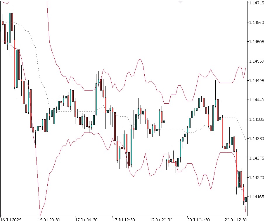
Fig. 1. The RobustBands indicator on price: a rolling median center with a half-width of k times 1.4826*MAD. On calm price this tracks a conventional Bollinger band closely; it separates from one only when an outlier enters the window.

RobustTrend: the Theil-Sen channel. This replaces the linear regression channel. The center is the Theil-Sen line evaluated at the current bar, and the channel half-width is robust as well, sized by the MAD of the residuals about that line via a small library helper, ResidualMadSigma(). Making the width robust too is the point: a classical regression channel widens the moment a spike enters, because it sizes itself on the residual standard deviation; the Theil-Sen channel keeps a steady width because it sizes itself on the residual MAD. The core loop reads the slope, the intercept, and the robust half-width:

      //--- Theil-Sen fit for the window ending at i, evaluated at the
      //--- newest bar, plus the robust residual half-width
      double slope   = g_robust.TheilSenSlope();
      double center  = g_robust.TheilSenIntercept(slope);
      double offset  = InpMultiplier * g_robust.ResidualMadSigma(slope, center);

      CenterBuffer[i] = center;
      UpperBuffer[i]  = center + offset;
      LowerBuffer[i]  = center - offset;

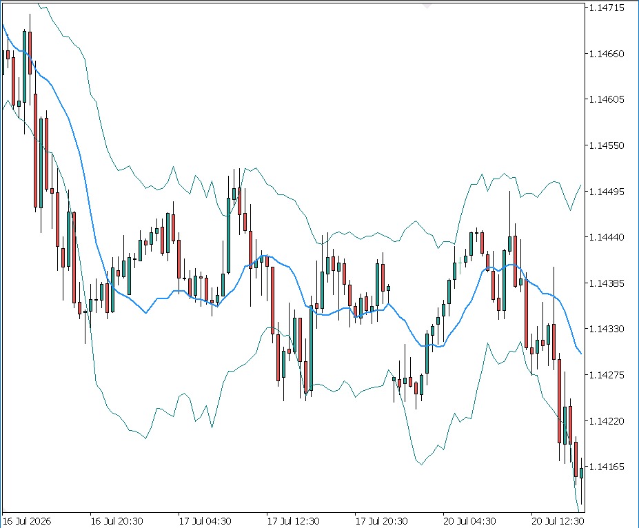
Fig. 2. The RobustTrend channel: a Theil-Sen center line with a residual-MAD half-width. Unlike a least-squares channel, a single spike in the window neither pivots the center line nor balloons the band.

RobustOscillator: the MAD-score. This replaces the z-score or sigma oscillator. It plots the robust z-score of the latest close against its window, (close - median) / (1.4826 * MAD), in a separate subwindow, with guide levels at plus or minus 2 and 3 that read like sigma bands because of the 1.4826 calibration. The advantage over a classical z-score is subtle but important: in a z-score oscillator, one spike inflates both the mean and the standard deviation, which shifts the zero line and compresses the reading of every other bar in the window. The MAD-score keeps its baseline steady, so the spike registers as a large reading on its own bar without distorting the bars around it. The entire per-bar computation is a single library call:

      //--- score this bar's close against the window it just completed
      ScoreBuffer[i] = g_robust.MadScore(close[i]);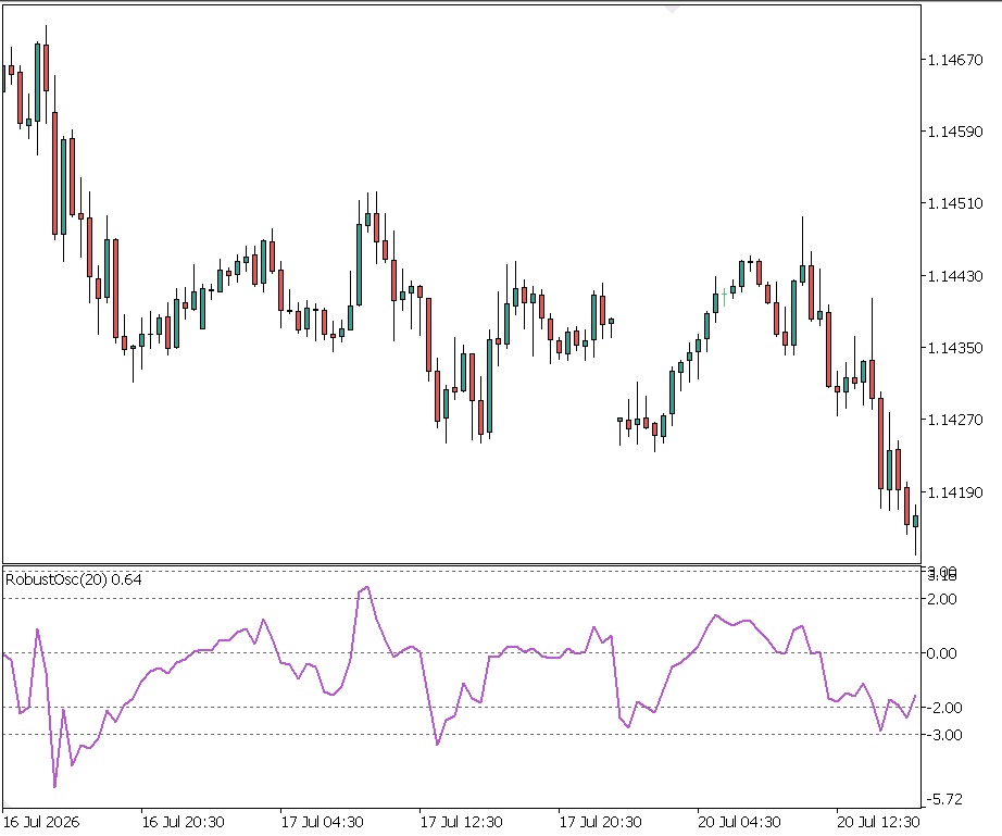

Fig. 3. The RobustOscillator subwindow: the MAD-score of the latest close. Guide lines at plus or minus 2 and 3 approximate sigma bands. A spike shows as its own large reading without dragging the baseline the surrounding bars are measured against.

Seeing the difference: the comparison overlay

The three indicators each replace one classical tool, but to see the replacement matter we need both tools on the same axis at once. The RobustComparison indicator draws two band pairs on price from a single shared window: the classical mean plus or minus k times StdDev, thin and gray, and the robust median plus or minus k times 1.4826*MAD, bold and colored. Crucially, both come from one ComputeAll() call over the same window, so any divergence is due purely to the estimator and not to a different period or price convention. This defends the comparison against the obvious objection, that the two bands were measured differently.

      if(!g_robust.ComputeAll(e))
       {
         ClearBar(i);
         continue;
       }

      //--- classical band: mean +/- k*StdDev
      double cls_off = InpMultiplier * e.stddev;
      ClsMidBuffer[i] = e.mean;
      ClsUpBuffer[i]  = e.mean + cls_off;
      ClsLoBuffer[i]  = e.mean - cls_off;

      //--- robust band: median +/- k*1.4826*MAD
      double rob_off = InpMultiplier * e.mad_sigma;
      RobMidBuffer[i] = e.median;
      RobUpBuffer[i]  = e.median + rob_off;
      RobLoBuffer[i]  = e.median - rob_off;

On a clean stretch of chart the two band pairs sit almost on top of each other, which is itself part of the story: the robust band is not a different indicator that happens to look similar, it is calibrated to agree with the classical one when the data is clean. The place to look is a spike or a gap. There, the gray classical band jumps and drifts, its mean pulled toward the outlier and its width inflated by it, while the colored robust band holds its position and width. That is the entire thesis of the article in a single screenshot.

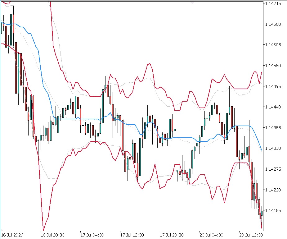
Fig. 4. The comparison overlay around a price spike. The gray classical band (mean plus or minus StdDev) balloons and drifts as the outlier enters its window; the colored robust band (median plus or minus 1.4826*MAD) barely moves. Both are computed over the same window.

The evidence: the breakdown point

A screenshot shows the effect; numbers prove it. The attached RobustContaminationDemo script measures the breakdown point directly on real price. It pulls the last N closed closes from the current chart, then progressively corrupts 0, 1, 2, ... bars with an outlier (sized relative to the window's own price range, so the test is meaningful on any symbol) and recomputes every estimator at each step. Reading down the resulting table shows the robust estimator holding flat while the classical one drifts on every added spike, and then the robust one finally tipping as the corrupted share approaches one half, the 50% breakdown point made literal.

The sweep is capped at N/2 on purpose: beyond 50% corruption even the robust estimators must break, which is precisely the concept being demonstrated. The measurement step is a single helper that feeds a fresh instance and calls ComputeAll():

//+------------------------------------------------------------------+
//| Feed an array of closes (chronological: [0] oldest) into a fresh |
//| library instance sized to the array length, and fill a full set  |
//| of estimates from it.                                            |
//+------------------------------------------------------------------+
bool Measure(const double &closes[], SRobustEstimates &e)
  {
   int n = ArraySize(closes);
   CRobustStats rs;
   rs.Init(n);
   for(int i = 0; i < n; i++)
      rs.Update(closes[i]);
   return(rs.ComputeAll(e));
  }

Run on EURUSD M30 with a 40-bar window and a spike of three times the window's price range, the script produces the table below. It is the central evidence of this article, so it is worth reading carefully. One caveat before the numbers: the script reads whatever history your terminal happens to hold at the moment you run it, so if you run it yourself your exact figures will differ from these, possibly by a lot on a different symbol, period, or day. That does not matter. It is the pattern down each column, robust holding while classical drifts, that reproduces, not the individual digits.

Corrupted	median	mean	MAD-sigma	StdDev	TS slope	OLS slope
0 (0%)	1.137980	1.138083	0.000556	0.000532	+0.000030	+0.000026
1 (2.5%)	1.138015	1.138275	0.000563	0.001304	+0.000030	-0.000002
3 (7.5%)	1.138130	1.138661	0.000608	0.001954	+0.000022	-0.000054
6 (15%)	1.138225	1.139239	0.000689	0.002588	+0.000003	-0.000121
10 (25%)	1.138395	1.140010	0.000778	0.003104	-0.000052	-0.000191
15 (37.5%)	1.138715	1.140974	0.001208	0.003424	-0.000203	-0.000245
18 (45%)	1.138995	1.141552	0.002039	0.003554	-0.000217	-0.000260
20 (50%)	1.142280	1.141937	0.005174	0.003610	-0.000217	-0.000263

Table 1. Breakdown sweep on EURUSD M30, 40-bar window, spike = 3x the window range. Selected rows from the full 0-to-20 sweep. Robust columns (median, MAD-sigma, TS slope) hold; classical columns (mean, StdDev, OLS slope) drift from the first spike.

Three things in this table carry the whole argument. First, and most striking, is the OLS slope on a single spike. At row 1, one corrupted bar out of forty flips the least-squares slope from +0.000026 to -0.000002, a sign change. The classical estimator has, on one bad tick, turned a rising trend into a falling one. The Theil-Sen slope on the same row is still +0.000030, unchanged, and does not even cross into negative territory until roughly 18% of the window is corrupted. One outlier is enough to reverse the classical trend reading; the robust one shrugs it off.

Second is the StdDev versus MAD-sigma pair. That same single spike inflates the standard deviation from 0.000532 to 0.001304, a jump of about 145%, while the robust MAD-sigma moves from 0.000556 to 0.000563, barely more than 1%. A band sized on StdDev would balloon on one bad tick; a band sized on MAD-sigma would not notice it. This is exactly the behavior the comparison overlay shows visually.

Third, and most elegant, is the breakdown point appearing in the data. Read the median column down: it barely moves for eighteen rows, drifting only within the window's own price range, and then at the very last row, 20 corrupted bars out of 40, exactly 50%, it jumps to 1.142280. The MAD-sigma does the same, holding near its clean value until it explodes to 0.005174 at 50%. This is not a bug and not a coincidence: it is the 50% breakdown point of the median, the theoretical limit, showing up precisely where the mathematics says it must. The estimator holds until, and only until, half the data is corrupted. The mean, by contrast, has already drifted steadily on every single row from the first spike onward, because its breakdown point is zero.

It is worth being precise about what happens at that final row, because a careful reader will notice it: at 50% corruption the MAD-sigma (0.005174) has not merely moved, it has overshot the classical StdDev (0.003610) that it beat comfortably on every earlier row. That is exactly right, and it is the honest edge of the story. The breakdown point guarantees the robust estimate stays bounded below half corruption; it promises nothing at half, where the deviations-from-median set is itself half spikes and the MAD tips hard. The robust estimator does not fail gracefully forever, it fails last. Everything it buys you is spent by the time the corruption reaches the boundary; the win is entirely in the eighteen rows before it.

Edge cases and pitfalls

A robust library is only as trustworthy as its behavior in the awkward corners. Several are worth stating plainly, both because they affect correct use and because they are the parts no reference will tell you.

Robust does not mean better returns. This is the most important caveat. Everything above concerns the statistical robustness of the estimators, their resistance to contamination, and the evidence proves exactly that and nothing more. It does not follow that a strategy built on robust indicators is more profitable than one built on classical indicators. On clean data the two are, by design, nearly identical; the robust version earns its keep specifically when outliers are present and when you would rather your indicator ignore them than react to them. Whether that is desirable depends entirely on the strategy. Do not read the breakdown-point evidence as a performance claim.

The Theil-Sen cost is real; keep the window modest. The pairwise-slope computation is O(n^2): a 40-bar window forms 780 slopes per evaluation, an 80-bar window forms 3160. For a per-bar indicator this is comfortably fast, but it grows quadratically, so a several-hundred-bar Theil-Sen window is a bad idea. The library pre-allocates the pair buffer once in Init() to avoid per-call allocation, but it cannot change the arithmetic. If you need a long-window robust slope, that is the point at which an approximate Theil-Sen algorithm becomes worth its complexity; for the windows an indicator actually uses, the exact O(n^2) version is the simplest correct choice.

The 50% ceiling is a ceiling, not a guarantee at 49%. The breakdown point says the estimate stays bounded below 50% corruption, not that it stays accurate. Table 1 shows the median drifting gently well before the 50% cliff, and the Theil-Sen slope degrading gradually from about 15% onward. Robust estimators buy you resistance to a minority of outliers; they do not make a window that is one-third garbage report the truth. If half your bars are bad, no estimator can help you, and the median simply fails last.

Even-length windows average two middle values. The median of an even-length window is the mean of its two central order statistics. That is the standard definition and the one the library uses, but it means a median can take a value that is not any actual price in the window, and it introduces a small, harmless dependence on window parity. It is worth knowing when you compare a median against the raw closes and find it landing between two of them.

Ties and flat windows. A perfectly flat window has a MAD of zero, which would make the robust z-score divide by zero. The library guards this explicitly in MadScore(), returning zero when MadSigma is not positive, so a dead-flat market yields a score of zero rather than a not-a-number. The same guard exists in the classical ZScore() for a zero standard deviation.

The input clamp drops bad bars; it does not repair them. Update() rejects a non-finite or non-positive close rather than storing it, which is the right default for the price series this library is built for and keeps a NaN out of every downstream sort. But rejecting is not the same as substituting: a rejected bar simply does not enter the window, so the ring holds one fewer real close than the bar index might suggest and Ready() stays false one bar longer. On normal FX and equity data this guard never fires. The one case to keep in mind is an instrument that can legitimately quote at or below zero, a spread series, or a differenced or de-based feed, where a non-positive value is real data, not corruption. There the c <= 0.0 half of the clamp is wrong for you and should be relaxed to a plain finiteness check.

Conclusion

We set out to replace the two numbers that quietly underpin most statistical indicators, the mean and the standard deviation, with estimators that do not fall apart when price misbehaves. The result is a compact toolkit built on one idea: the median and the quantities derived from it (MAD, Theil-Sen slope) have a high breakdown point, so a minority of bad ticks cannot drag them, while the mean, the standard deviation, and the least-squares slope have a breakdown point of zero and can be moved without limit by a single outlier. Concretely, the article delivers:

1. RobustStats.mqh, the shared library. A single class, CRobustStats, computing the robust estimators (median, MAD, MadSigma, MadScore, Theil-Sen slope and intercept, residual MAD) and their classical twins (mean, StdDev, z-score, OLS slope and intercept) over one ring-buffered window, plus a one-pass ComputeAll().
2. Three drop-in indicators. RobustBands (median plus or minus 1.4826*MAD, replacing Bollinger), RobustTrend (a Theil-Sen channel with a residual-MAD width, replacing the linear regression channel), and RobustOscillator (the MAD-score, replacing the z-score oscillator). Each is a thin shell over the library with correct warm-up handling.
3. The comparison overlay and the breakdown-point script. RobustComparison draws the classical and robust bands together from one shared window so the difference is visible on the candles; RobustContaminationDemo measures the breakdown point on real price and prints it as a table.

The evidence closed the loop the article set out to close. On real EURUSD data, one corrupted bar out of forty flipped the sign of the least-squares slope and inflated the standard deviation by 145%, while the Theil-Sen slope and the MAD held steady; and the median's theoretical 50% breakdown point appeared exactly where the mathematics predicted, holding flat until half the window was corrupted and only then giving way. The estimators behave precisely as robust statistics says they should.

The engineering lessons carry beyond these specific indicators. Keep a single source of truth so the visual tools and any consumer can never diverge; verify numerical code against known answers before building on it; and understand the O(n^2) cost you are paying for an exact Theil-Sen estimator so you choose the window deliberately. Most of all, know what your evidence proves and what it does not: this toolkit is demonstrably robust to contamination, which is a statistical property, not a promise of profit. Take these as reliable building blocks, drop them in wherever a mean or a standard deviation is quietly assuming the data is clean, and test what they do to your own strategy on your own terminal before drawing any trading conclusion.

File	Type	Description
RobustStats.mqh	Library	The CRobustStats class: median, MAD, MadSigma, MadScore, Theil-Sen slope and intercept, residual MAD, and the classical twins (mean, StdDev, z-score, OLS slope and intercept), with a one-pass ComputeAll().
RobustBands.mq5	Indicator	Median plus or minus k times 1.4826*MAD bands, a robust replacement for Bollinger Bands.
RobustTrend.mq5	Indicator	Theil-Sen trend channel with a residual-MAD half-width, a robust replacement for the linear regression channel.
RobustOscillator.mq5	Indicator	MAD-normalized oscillator (the robust z-score), a replacement for the z-score / sigma oscillator, plotted in a subwindow.
RobustComparison.mq5	Indicator	Overlays the classical (mean plus or minus StdDev) and robust (median plus or minus 1.4826*MAD) bands on price from one shared window for a direct visual comparison.
RobustContaminationDemo.mq5	Script	Measures the breakdown point on real chart data: pulls N closes, progressively corrupts them, and prints the robust-versus-classical estimates as a table.
MQL5.zip	Archive	Archive with all files above. Unpack it into the terminal installation directory and every file is placed in its required location.