Learnable Curves, Not Weights: A Kolmogorov-Arnold Network from Scratch

Contents

1. Introduction
2. What the finished tool does
3. From weights to curves: what a KAN is
4. The B-spline foundation
5. The learnable edge, layer, and network
6. Training by least-squares
7. Proving the network learns
8. From price to features
9. The indicator: prediction and readable curves
10. The Expert Advisor and an out-of-sample test
11. Conclusion

Introduction

A standard neural network learns a number on every connection. The signal flowing along an edge is the input multiplied by that fixed weight, and each neuron then passes the sum through one fixed nonlinearity, a sigmoid or a ReLU. The shape of the nonlinearity is chosen by the developer, never learned. The network only adjusts how much of it to use.

A Kolmogorov-Arnold Network turns that around. There are no scalar weights and no fixed activation. Every edge carries its own small function, a curve that the training process shapes. A neuron simply sums the outputs of the edge functions feeding into it. The network learns the shapes themselves, and because each shape is a function of one input, you can plot it and read what the model decided that input means.

That last property is the reason this is worth building for trading. A conventional model that predicts the next bar is a black box. A KAN, by contrast, gives you a picture: the curve on the RSI edge shows exactly how the model expects RSI to bend the forecast, and the curve on the volatility edge shows the same for ATR. You are not left guessing what the network keyed on.

This article is a full, self-contained build. We implement the B-spline basis using the De Boor-Cox recursion, assemble the edges, layers, and network, and fit the model with a direct least-squares solve instead of gradient descent. This removes learning-rate tuning and gradient-related failure modes. We then feed the network four market features, save the trained model, draw its learned curves on the chart, and trade its prediction in the Strategy Tester. The code is written first and tested against a fixed standard, and the article is written around what the tests actually produced.

What the finished tool does

Before the math, here is the result. The trained network runs as an indicator in a separate window under the chart. Each closed bar produces a predicted next-bar return, drawn as a colored histogram, green when the model expects the next bar up and red when it expects down. Above it, anchored to the corner of the chart, sits a small panel with one curve for each input feature. Those curves are the functions the network learned, and they do not move tick to tick: they are the model.

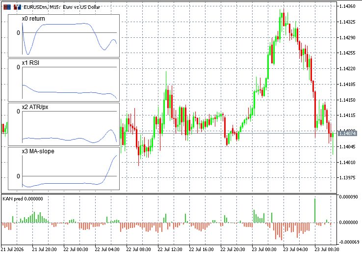
Fig. 1. The indicator: a next-bar-return histogram in a separate window, and the learned edge-curves in a corner panel

The same model drives an Expert Advisor. On EURUSD M15, over a five-month window that the model never saw during training, the strategy returned a small but genuine profit with a shallow drawdown. The exact figures are in the final section, presented as they came out of the tester. The point of the early look is honesty about scope: this is a first working KAN on the platform and a readable one, not a profit engine.

The system is a short pipeline. Price bars become four features. The features are normalized into the spline domain, the network predicts the next-bar return, and a threshold turns that prediction into a trade. The same trained model feeds both the indicator, which draws the curves, and the Expert Advisor, which trades the prediction. The diagram below is that flow.

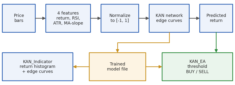
Fig. 2. The pipeline: bars become features, the network turns features into a predicted return, and a threshold turns that into a trade. One trained model feeds both the indicator and the Expert Advisor

Each block in that diagram is a class or a program in the attached files, and the rest of the article walks them in the order the pipeline runs. The library splits along the same lines: the basis and the network are pure math with no market knowledge, the feature builder is the only piece that touches price, and the store, indicator, and Expert Advisor are the plumbing that turns a trained model into something you run.

From weights to curves: what a KAN is

Write a single dense layer in the usual way. For output node j, the layer computes a weighted sum of its inputs and applies one activation:

y[j] = act( sum over i of w[i][j] * x[i] )

The weights w[i][j] are learned. The function act is fixed. A KAN layer computes something structurally different:

y[j] = sum over i of phi[i][j]( x[i] )

There is no outer activation and there are no scalar weights. Each edge from input i to output j carries its own univariate function phi[i][j], and the node just sums them. All the learning lives in the shapes of those functions. The diagram below places the two approaches side by side: on the left, a weight is a number and the nonlinearity sits in the node; on the right, the nonlinearity lives on the edge and is learned.

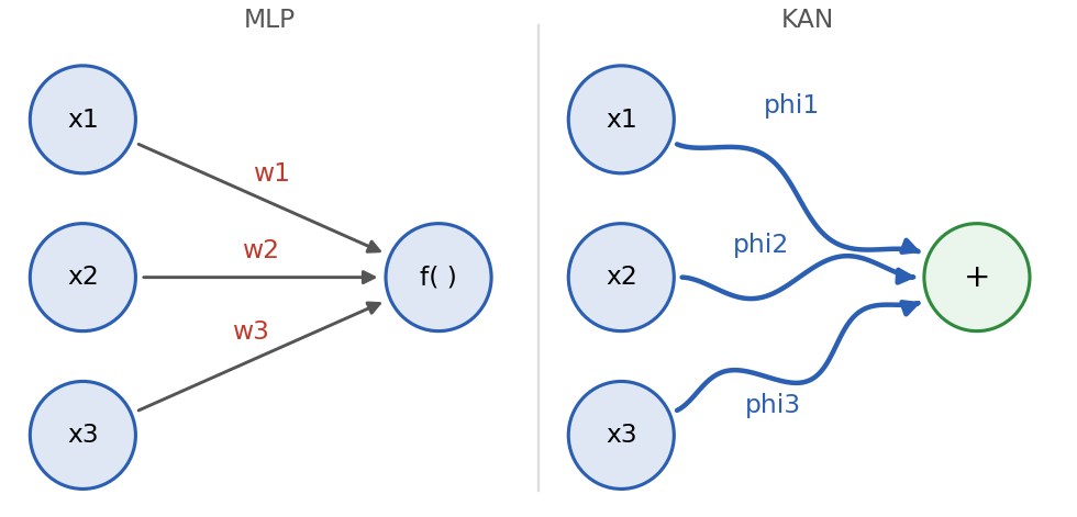
Fig. 3. A standard edge carries one weight and the node applies a fixed activation. A KAN edge carries a learnable curve and the node only sums

The practical difference is expressiveness per connection. A scalar weight can only scale its input, so a single edge is a straight line through the origin, and the network needs depth and many neurons to bend that into a curve. A KAN edge is already a curve, so a single edge can represent a relationship that rises, flattens, and falls again. For market inputs this matters, because the effect of RSI on the next bar is not a straight line: the extremes near 20 and 80 behave differently from the middle, and one KAN edge can hold that whole shape.

To make a function on an edge learnable, it needs a representation with a handful of adjustable numbers that can bend it into many shapes. We use a spline. Each edge function is written as a weighted sum of fixed basis functions:

phi(x) = sum over b of c_b * B_b(x)

The basis functions B_b(x) are fixed once the grid is chosen. The coefficients c_b are what the edge learns. This choice has a consequence that shapes the whole design: phi is linear in the coefficients c_b, even though it is a curved function of x. A model that is linear in its unknowns can be fit by least-squares, in one direct solve, with no iteration. That is why this KAN needs no gradient descent.

The B-spline foundation

Everything rests on the basis functions B_b(x), so they are built and tested first. The class CBSpline owns only the basis: the knot vector and the evaluation of each B_b(x) at a given point. It can also compute the weighted sum once coefficients are supplied. The coefficients themselves live one level up, in the edge.

A cubic B-spline of degree k over a domain [a, b] is defined on a knot vector. We split [a, b] into G equal intervals and use a clamped knot vector, repeating each endpoint k+1 times. The clamp has two useful effects: the basis functions sum to exactly 1 across the whole closed domain, and the curve interpolates its end control points. With G intervals and degree k there are G + k basis functions, which is the number of coefficients each edge carries.

The heart of the class is the evaluation of the basis at a point. The De Boor-Cox recursion builds, from the innermost degree outward, the k+1 basis functions that are non-zero on the span containing x. Every other basis function is exactly zero there, so the output array is zeroed first and only the active entries are filled.

//+------------------------------------------------------------------+
//| Evaluate all basis functions at x (De Boor - Cox recursion)      |
//|                                                                  |
//|  Only k+1 basis functions are non-zero on any span; the rest of  |
//|  out[] is zeroed. The recursion builds them without dividing by  |
//|  a zero-width knot interval (the clamp creates repeated knots),  |
//|  guarding each denominator.                                      |
//+------------------------------------------------------------------+
bool CBSpline::BasisEval(double x, double &out[]) const
  {
   if(m_nBasis <= 0)
     {
      Print("CBSpline::BasisEval - not initialized");
      return false;
     }
   if(ArraySize(out) != m_nBasis)
      ArrayResize(out, m_nBasis);
   ArrayInitialize(out, 0.0);
//--- clamp input into the domain
   if(x < m_a)
      x = m_a;
   if(x > m_b)
      x = m_b;
   const int k  = m_degree;
   const int mu = FindSpan(x);
//--- local basis values N[0..k] for the active span, plus scratch
//    left[j]  = x - knots[mu + 1 - j]
//    right[j] = knots[mu + j] - x
   double N[];
   double left[];
   double right[];
   ArrayResize(N,     k + 1);
   ArrayResize(left,  k + 1);
   ArrayResize(right, k + 1);
   N[0] = 1.0;
   for(int j = 1; j <= k; j++)
     {
      left[j]  = x - m_knots[mu + 1 - j];
      right[j] = m_knots[mu + j] - x;
      double saved = 0.0;
      for(int r = 0; r < j; r++)
        {
         double denom = right[r + 1] + left[j - r];
         double term  = (denom != 0.0 ? N[r] / denom : 0.0);
         N[r]  = saved + right[r + 1] * term;
         saved = left[j - r] * term;
        }
      N[j] = saved;
     }
//--- scatter the k+1 local values into global basis positions.
//    the active basis functions are B_{mu-k} .. B_{mu}
   const int base = mu - k;
   for(int j = 0; j <= k; j++)
     {
      int gi = base + j;
      if(gi >= 0 && gi < m_nBasis)
         out[gi] = N[j];
     }
   return true;
  }

The inner loop is the recursion. The guard denom != 0.0 matters because the clamped knot vector deliberately repeats knots at the endpoints, which creates zero-width intervals that would otherwise divide by zero. The final loop scatters the k+1 local values into their global positions in the output array, so a caller reading out sees the value of every basis function, most of them zero.

To see the basis itself, the script KAN_Export_Basis.mq5 samples every B_b(x) across the domain and writes them to a CSV, which a short Python script plots. The figure below is that output for a grid of 8 intervals at degree 3, the exact configuration used in this build.

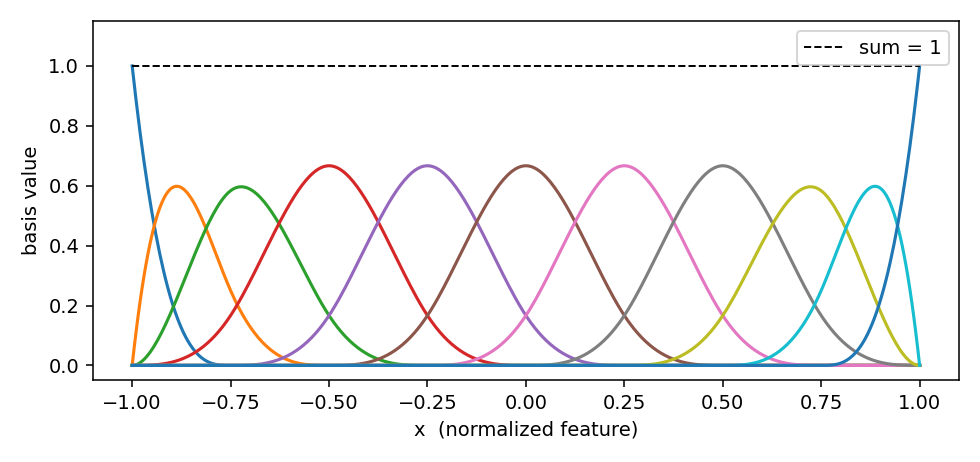
Fig. 4. The eleven cubic basis functions for a grid of 8 intervals; each is local, and at every point they sum to 1, the dashed line

Each bump is one basis function. They overlap, each is non-zero only on a local stretch of the domain, and at every point they add up to 1, the dashed line. A curve is built by giving each bump a height, the coefficient, and adding them. Because the bumps are local, moving one coefficient bends the curve only in that region, which is what lets an edge learn a shape that behaves differently for low RSI than for high RSI.

The second figure makes that concrete. It takes the same basis, scales each bump by a coefficient, and sums the scaled bumps into a single curve. The faint lines are the scaled bumps, and the bold line is their sum, which is exactly what one KAN edge computes for a given input. The coefficients here are illustrative, chosen to show the mechanism, but the shape is produced the same way for a trained edge: the fit sets the coefficients, and the coefficients set the curve.

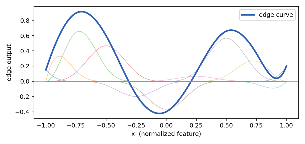
Fig. 5. Each bump scaled by its coefficient, faint, and their sum, bold; that sum is what one edge computes for a given input

Notice the leverage this gives the fit. There are only eleven numbers to set per edge, yet they place a smooth curve anywhere within the domain. That small, linear set of unknowns is what makes the whole layer solvable in one step, which is the subject of the training section. It also keeps the model compact: four edges of eleven coefficients is a model of forty-four numbers, small enough to save as a short text file and reload in an instant.

The learnable edge, layer, and network

With the basis in hand, the network is three small classes stacked on top of it. An edge holds a coefficient vector and nothing else. A layer holds a grid of edges and one shared basis. The network holds a layer plus the normalization that maps raw features into the basis domain.

The edge, CKANEdge, is deliberately thin. It stores its coefficients, and its forward evaluation is the weighted sum of the basis at x. The basis is not duplicated per edge; it is owned by the parent layer and passed in on each call, so every edge in a layer shares one knot vector.

The layer, CKANLayer, is where the KAN definition becomes code. Its forward pass evaluates the basis functions at each input once, then for every output node adds up the contribution of each incoming edge:

//+------------------------------------------------------------------+
//| Forward pass:  y[j] = sum_i phi[i][j](x[i])                      |
//+------------------------------------------------------------------+
void CKANLayer::Forward(const double &x[], double &y[]) const
  {
   if(ArraySize(y) != m_nOut)
      ArrayResize(y, m_nOut);
   ArrayInitialize(y, 0.0);
//--- evaluate the basis functions at each input once, reuse across all outputs
   double basis[];
   for(int i = 0; i < m_nIn; i++)
     {
      m_basis.BasisEval(x[i], basis);
      for(int j = 0; j < m_nOut; j++)
        {
         const CKANEdge *e = GetPointer(m_edge[EdgeIdx(i, j)]);
         double s = 0.0;
         for(int b = 0; b < m_nBasis; b++)
            s += e.Coef(b) * basis[b];
         y[j] += s;
        }
     }
  }

Compare this to a dense layer. There is no call to any activation function, and there is no weight matrix. The nested sum over b is the edge evaluating its own curve, and the sum over i adds those curves at the output node. Evaluating the basis once per input and reusing it across all outputs keeps the cost down when the network is wider than one output.

The network, CKAN, wraps a single layer and a per-feature normalization. The basis is defined on a fixed domain, minus one to one by default, but raw features like RSI live on their own scales. Before the layer sees them, each feature is mapped from its training minimum and maximum into the domain and clamped there. Without this step the splines would be asked to evaluate outside their knots and extrapolate, which produces meaningless output. The normalization is learned from the training data and saved with the model, so the live features are mapped exactly as they were during training.

Training by least-squares

Because each edge is linear in its coefficients, fitting a layer is a linear least-squares problem, not an optimization loop. For a single output the model is:

y = sum over i and b of c[i][b] * B_b( x[i] )

Stacking the basis of every input side by side turns this into one design matrix A, where each row is a training sample and each block of columns holds the basis values of one input. The coefficients that best fit the targets are the solution of the normal equations:

( A^T A + lambda I ) c = A^T y

The term lambda I adds ridge regularization on the diagonal. B-spline design matrices are often nearly singular because some basis functions are rarely active on the sampled inputs. The ridge term keeps the system solvable. The matrix A^T A depends only on the inputs, so it is built once and reused across output columns; only the right-hand side changes per output. The solve itself is a Cholesky factorization, which is exact for the symmetric positive-definite system the ridge guarantees. The layer's fit routine builds the design matrix, forms the normal equations, and scatters the solved coefficients back into the edges:

//--- The Gram matrix M = A^T A + lambda I depends only on A, so it is
//    the same for every output column. Build it once and reuse it; only
//    the right-hand side g = A^T y[:,j] changes per output.
   double M[];
   double g[];
   double yCol[];
   double c[];
   ArrayResize(yCol, rows);
   CKANSolve::GramMatrix(A, rows, n, lambda, M);
   for(int j = 0; j < m_nOut; j++)
     {
      //--- extract target column j and form g = A^T y[:,j]
      for(int r = 0; r < rows; r++)
         yCol[r] = Y[r * m_nOut + j];
      CKANSolve::RhsAtY(A, yCol, rows, n, g);
      if(!CKANSolve::SolveSPD(M, g, n, c))
        {
         PrintFormat("CKANLayer::FitLSQ - solve failed for output %d", j);
         return false;
        }
      //--- scatter c back: c[i*nBasis + b] -> edge(i,j) coefficient b
      for(int i = 0; i < m_nIn; i++)
         for(int b = 0; b < m_nBasis; b++)
            m_edge[EdgeIdx(i, j)].SetCoef(b, c[i * m_nBasis + b]);
     }

This excerpt is the core of FitLSQ; the lines that build the design matrix A from the input rows come just above it in the source. The fit is deterministic. Run it twice on the same data and you get identical coefficients, because there is no random initialization and no learning rate to tune. That determinism is what makes the network testable to a fixed tolerance, which is the subject of the next section.

The trade-off is worth stating plainly. A direct least-squares solve fits one layer exactly, so this build uses a single expressive layer rather than a deep stack. That is not a limitation for the task here, because a KAN concentrates its power in the width of its edges, not in depth: each edge is already a full curve, and four inputs mapping to one output through four independent curves is a rich model of an additive relationship. A deeper KAN would need gradient descent to train, which trades the exact, reproducible solve for learning rates and gradient checks. For a first, verifiable build, the exact solve is the right choice, and the class still stores its structure so a deeper network can forward-pass if a later experiment calls for one.

Proving the network learns

A model that cannot reproduce a function you already know is not worth pointing at a market. The library ships two test scripts that make the claim concrete, and both must pass before anything touches price data.

The first, KAN_BSpline_Test.mq5, checks the basis alone. It sweeps points across the domain and confirms three properties: the basis functions sum to 1 everywhere, none is negative, and the basis reproduces a straight line exactly, which a correct B-spline must. It also checks that all-ones coefficients produce the constant 1, a direct consequence of the partition-of-unity property. On the default grid the script reports:

===== CBSpline Level-1 Verification =====
G=8  k=3  domain=[-1.00, 1.00]  samples=401
NumBasis = 11  (expect G+k = 11)
Max |sum Bi - 1|   = 0.000e+00
Min basis value    = 0.000e+00
Max |f(x) - x|     = 2.220e-16
RESULT: 9 PASS, 0 FAIL

The line that matters most is the reproduction of a straight line to 2.2e-16, machine precision. That confirms the recursion, the knot vector, and the coefficient handling are all correct, because a single error in any of them breaks linear reproduction.

The second, KAN_Test.mq5, checks the whole network. It fits a single edge to sin(3x), then fits a two-input network to sin(3 * x0) + x1 * x1, and finally confirms that saving and reloading the coefficients gives identical predictions. The additive case is the signature KAN test: a sum of one-variable functions is recovered exactly, each on its own edge, which a plain linear model cannot do. The script reports:

===== KAN Level-2 Verification =====
--- Proof 1: fit y = sin(3x), single edge ---
  max |KAN(x) - sin(3x)| = 3.7e-04
--- Proof 2: fit y = sin(3*x0) + x1^2, additive 2->1 ---
  max |KAN - (sin(3*x0)+x1^2)| = 6.1e-04
--- Proof 3: save / reload roundtrip ---
  max |pred_a - pred_b| = 0.000e+00
RESULT: 3 PASS, 0 FAIL

The fit errors are on the order of a few parts in ten thousand, set by how finely the grid samples the target, and the roundtrip is exact. With the basis and the network both verified, the design is sound, and the remaining work is to feed it market data.

From price to features

The network needs numeric inputs and a target. One class, CKANFeatures, produces both, and it is shared by the trainer, the indicator, and the Expert Advisor. Sharing matters: if the trainer computed features one way and the live EA another, the model would see inputs it was never trained on and its output would be noise. Writing the computation once removes that whole class of bug.

The four features are chosen so each carries a distinct piece of market information: a one-bar return for momentum, RSI for the oscillator state, ATR divided by price for relative volatility, and the slope of a fast moving average for trend. The build routine reads them for a given bar shift and fills the feature row:

//--- indicator reads: two MA values for the slope, one RSI, one ATR.
//    Set the receiving arrays as-series so index i means "i bars back",
//    matching the shifts above (ma[0]=shift, ma[1]=shift+1).
   double rsi[], atr[], ma[];
   ArraySetAsSeries(rsi, true);
   ArraySetAsSeries(atr, true);
   ArraySetAsSeries(ma,  true);
   if(CopyBuffer(m_hRSI, 0, shift, 1, rsi) != 1)
      return false;
   if(CopyBuffer(m_hATR, 0, shift, 1, atr) != 1)
      return false;
   if(CopyBuffer(m_hMA,  0, shift, 2, ma)  != 2)
      return false;
// ma[0] = MA at shift, ma[1] = MA at shift+1
//--- x0: one-bar return
   feat[0] = (c0 - c1) / c1;
//--- x1: RSI raw 0..100
   feat[1] = rsi[0];
//--- x2: ATR relative to price
   feat[2] = atr[0] / c0;
//--- x3: MA slope, price-normalized (newer minus older)
   feat[3] = (ma[0] - ma[1]) / c0;

The as-series calls are the detail that catches people. MQL5 fills copy buffers oldest-first by default, so reading two moving-average values and subtracting them the wrong way round would flip the sign of the slope. Setting the receiving arrays as-series makes index zero the most recent bar, so ma[0] - ma[1] is the newer value minus the older one, a positive slope in an uptrend. The prediction target, built only by the trainer, is the next bar's return, which keeps the fit a plain regression.

The trainer, KAN_Train.mq5, walks the history, collects feature rows and their targets, fits the network, and saves the model. It also reports honest in-sample diagnostics and verifies the save. On EURUSD M15 over three thousand bars, a representative run reported an in-sample correlation between prediction and actual return of about 0.21 and a directional accuracy near 52 percent, with the save-and-reload check matching to 3e-15. Those numbers are modest by design: next-bar return is mostly noise, and a small, honest in-sample signal is what a real market gives. The saved model is written to the shared common folder so the Strategy Tester, which sandboxes each agent's own files, can read the same file the live terminal wrote.

The indicator: prediction and readable curves

The indicator, KAN_Indicator.mq5, does two things. It loads the saved model and, on each closed bar, plots the predicted next-bar return as a colored histogram in a separate window. It also draws the learned edge-curves in a small panel anchored to the corner of the chart. The prediction is the model at work; the curves are the model itself.

The curves are rendered once with the Canvas library into a bitmap that is pinned to a screen corner. This is a deliberate choice. A bitmap label anchored to a chart corner does not move when you scroll or zoom, so there is nothing to redraw on every chart event and nothing to flicker. The panel is built in OnInit and left alone, and each feature gets its own cell with a zero line, a short axis, and the curve sampled across the feature's trained range.

Reading the panel is the whole point of using a KAN. A cell whose curve slopes down from left to right says the model expects that feature to bend the forecast lower as it rises. A cell whose curve is nearly flat says the model found little use for that feature. A cell with a bend or a hump says the relationship is genuinely non-linear, high and low values pushing the same direction while the middle does something else. None of that is available from a network of scalar weights, and it is drawn straight from the coefficients the fit produced.

The colors, fonts, and panel geometry are all inputs, so the panel stays readable on any chart background. On a white background, a dark curve color and a black label read cleanly; on a dark theme, lighter values work better. The prediction histogram has its own up and down colors as inputs as well.

The indicator and the Expert Advisor both load the model from a text file written by the trainer, and that file is the reason the two agree. The store writes the geometry, the per-feature normalization, and every coefficient to a plain text file with one value per line, which sidesteps the tab separators that the built-in write inserts between multiple arguments. Reloading is the exact inverse. The trainer confirms this by reading the model back after saving and verifying that predictions match within a rounding error (~1e-15). That check is not decoration. If the saved model did not reconstruct exactly, the curves you read on the chart would not be the curves the Expert Advisor trades.

The file is written to the shared common folder rather than the terminal-local one. The Strategy Tester runs each agent in its own sandbox with a private files directory, so a model saved to the local folder is invisible to a tester run, and the Expert Advisor would fail to load it. The common folder is reachable from both the live terminal and every tester agent, so one trained model serves the chart and the backtest without copying anything by hand.

The Expert Advisor and an out-of-sample test

The Expert Advisor, KAN_EA.mq5, trades the same prediction. It loads the model, and on each new bar it rebuilds the features through the shared class, reads the network's forecast, and acts only when the forecast clears a threshold. The threshold filters out the many near-zero predictions where the model has no real opinion. Stops and targets scale with ATR, so they widen in volatile conditions and tighten in quiet ones, and the size is a fixed lot to keep the tester result about the signal rather than about money management.

//+------------------------------------------------------------------+
//| Tick handler: act once per new bar                               |
//+------------------------------------------------------------------+
void OnTick()
  {
   if(!g_ready) return;
//--- run only on a freshly opened bar
   datetime barTime = iTime(_Symbol, _Period, 0);
   if(barTime == g_lastBar) return;
   g_lastBar = barTime;
//--- build features for the last closed bar (shift 1) and predict
   double feat[]; double yout[];
   if(!g_feats.Build(1, feat)) return;
   g_net.Predict(feat, yout);
   double pred = yout[0];
//--- decide direction from the thresholded prediction
   int dir = 0;                  // +1 buy, -1 sell, 0 no signal
   if(pred >  InpThreshold) dir = +1;
   if(pred < -InpThreshold) dir = -1;
//--- current position state
   bool isBuy = false;
   bool have  = HasPosition(isBuy);
   if(dir == 0)
      return;                    // weak prediction: leave things as they are
   if(!have)
     {
      OpenTrade(dir > 0);
      return;
     }
//--- a position exists: if the signal agrees, hold; if it opposes,
//    close (and optionally reverse) so the book follows the model.
   bool signalIsBuy = (dir > 0);
   if(signalIsBuy != isBuy)
     {
      g_trade.PositionClose(_Symbol);
      if(InpReverse)
         OpenTrade(signalIsBuy);
     }
  }

Acting once per new bar is intentional. The features are computed on closed bars and the model was trained on bar-level data, so evaluating every tick would only add noise and cost. When a position is already open and the model flips, the EA closes it and, if reversing is enabled, opens the opposite side, so the book follows the current forecast rather than a stale one.

The honest test is out-of-sample. The model was trained on recent history, so the tester was run on an earlier window the model never saw, EURUSD M15 from the first of January to the first of June 2026, on real ticks. Running it on the same bars the model trained on would flatter the result and prove nothing. The tester produced the following:

Metric	Value
Test period (out-of-sample)	2026.01.01 - 2026.06.01, EURUSD M15, real ticks
Initial deposit	10 000.00 USD
Total net profit	131.45
Profit factor	1.05
Expected payoff	0.42
Sharpe ratio	0.74
Maximal balance drawdown	238.79 (2.36%)
Total trades	310
Profit trades	132 (42.58%)
Average profit / average loss	22.25 / -15.76

The picture is a small, positive edge. The win rate is under half, at 42.58 percent, but the average win of 22.25 is larger than the average loss of 15.76, and that gap is what carries the profit factor above 1. The drawdown stayed shallow at 2.36 percent, which is the ATR-scaled stops doing their job. This is not a system to trade a live account on as-is; it is evidence that a four-feature KAN, fit by least-squares on next-bar return, captured a real if modest structure in unseen data. The balance curve over the test is below.

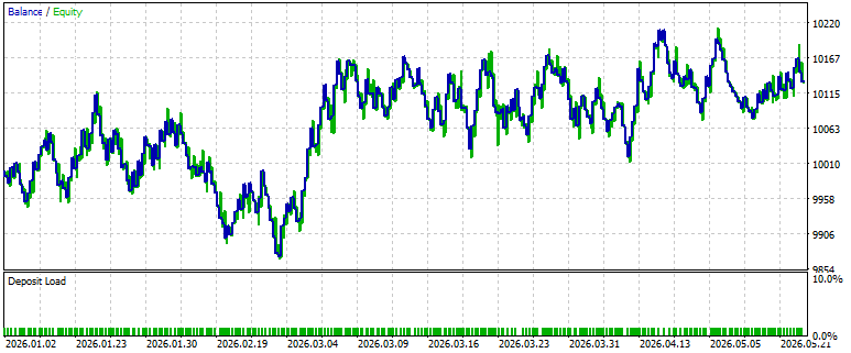
Fig. 6. The balance curve over the out-of-sample test, EURUSD M15 from January to June 2026

Conclusion

We built a Kolmogorov-Arnold Network in MQL5 from the ground up. The B-spline basis is written with the De Boor-Cox recursion and verified to machine precision, the edges and layer implement the sum-of-curves definition directly, and the whole layer is fit by a single least-squares solve with no gradient descent. The network was checked against known functions before it saw a price, then trained on four market features, drawn on the chart as the curves it learned, and traded through an Expert Advisor on an out-of-sample window.

What you can run from the attached files:

• Compile and run KAN_BSpline_Test.mq5 and KAN_Test.mq5 to reproduce the verification, 9 and 3 passes with no failures.
• Run KAN_Train.mq5 on a chart to fit a model and write it to the common folder.
• Attach KAN_Indicator.mq5 to see the live prediction and the learned-curve panel.
• Load KAN_EA.mq5 in the Strategy Tester on a window outside the training data to measure it out-of-sample.

The most useful next step for a reader is to change the feature set and retrain. Because the fit is a direct solve and the curves are plotted, you get immediate, readable feedback on whether a new input carries signal: train, attach the indicator, and look at the shape of its curve. A flat curve is a feature the model ignored, and a bent one is a feature it found a use for.

#	Filename	Type	Description
1	BSpline.mqh	Include	Cubic B-spline basis, De Boor-Cox evaluation
2	KANSolve.mqh	Include	Ridge-regularized normal equations, Cholesky solver
3	KAN\KAN.mqh	Include	Edge, layer, and network with least-squares fit
4	KAN\KANFeatures.mqh	Include	Shared market feature and target builder
5	KAN\KANStore.mqh	Include	Save and load a trained model to the common folder
6	KAN_BSpline_Test.mq5	Script	Level-1 verification of the basis
7	KAN_Test.mq5	Script	Level-2 verification of the network
8	KAN_Train.mq5	Script	Fit a KAN to history and save the model
9	KAN_Export_Basis.mq5	Script	Export the basis functions to CSV for plotting
10	KAN_Indicator.mq5	Indicator	Live prediction and learned-curve panel
11	KAN_EA.mq5	Expert	Trades the network prediction with ATR-scaled stops
12	plot_kan_basis.py	Python	Plots the exported B-spline basis functions
13	MQL5.zip	Archive	Archive with all project files in their subfolders; unpack it into the terminal data directory and every file lands in its required location