Trading Options Without Options (Part 4): More Complex Option Strategies

Introduction

The theory of options trading is based on the Black–Scholes formula, which, in turn, is based on the assumption that the movement of the underlying asset follows a random process with a normal distribution of price increments. This assumption is clearly refuted by empirical evidence (see Fig. 1), which means that the theory as a whole is incorrect.

For comparison, Fig. 1 shows distribution curves of price changes for a normal distribution (Normal distribution — dark blue line) and the empirical average distribution with “fat tails” (“Fat tail” distribution — dark green line) for an arbitrary underlying asset. There is a fundamental difference between them — mainly in the region of large price changes. The y-axis shows the frequency of occurrence of the corresponding price increments within the interval specified on the x-axis.

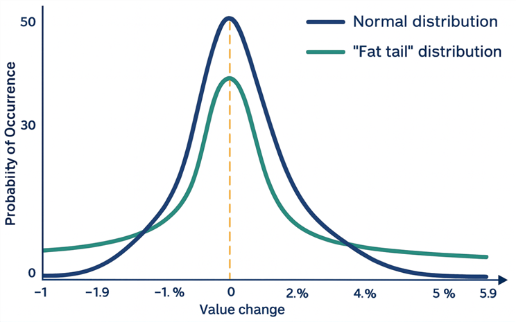
Fig. 1. Comparison of the normal distribution of price increments and the actual distribution with “fat tails.”

In addition, market data exhibits fractal properties (self-similarity). This means that the charts for a day, a week, or a month are structurally similar. This property clearly does not fit within the framework of a simple random walk.

Finally, there is a phenomenon known as historical volatility clustering. This phenomenon cannot be described by the distribution over a single time interval alone, but it is important for understanding the dynamics. Historical volatility is not constant: periods of high volatility tend to cluster together. The same is true of periods of low volatility. A strong move is usually followed by a series of other strong moves. This completely contradicts the hypothesis that asset price increments are independent.

We will attempt to test this phenomenon (historical volatility clustering) and apply it to options trading in the next article in this series.

The fact that a theory is flawed does not mean that it cannot be used in practice. At least in part. In the vast majority of cases, the so-called “fat tails” are driven by news events, which cannot always be predicted in advance — or, more accurately, almost never can be. Therefore, if they are included in the calculation of, for example, historical volatility (HV), the average profit will be underestimated and may no longer offset the losses from “fat tails.” Therefore, it is more appropriate to limit such risks. This will be discussed later.

Level-based Expiration of an Option Structure for Strategies Based on Long Options

In the previous article, among other things, we discussed option strategies based on long options. During practical testing, it became clear that it would be advisable to close out the option structure early when the price of the underlying asset reaches a statistically justified level (here and below, this refers to the rebalancing levels of the option structure).

In real-world options trading, this is not always possible due to limited liquidity in such cases (this is particularly true on the MOEX exchange). When emulating options, there are generally no liquidity problems with early expiration. Let's add this feature to our Expert Advisor (EA).

To begin, let's add an input parameter specifying the option level number at which the structure should be closed at which the option structure should be closed out early. It is an integer greater than zero. Also, let's add a flag to control whether to enable or disable the level-based expiration mode. With the settings shown below, the option structure will close at the seventh option level.

// ---------------------------------------------------------------------
input bool      UseExpirationPriceLevel = true;                       // Use Expiration Price Level
input int       ExpirationPriceLevel = 7;                             // Expiration Price Level
// ---------------------------------------------------------------------

Now let's upgrade our Expert Advisor (EA). If level-based expiration is enabled, then when the option structure's rebalancing level increases, we check its number and, if it has reached the value specified for expiration, close the positions and stop trading until the next day. This algorithm is shown in the code below (the complete code is in the file Article4-OptionTrader.mq5).

// ---------------------------------------------------------------------
//      Check whether options should be expired early:
// ---------------------------------------------------------------------
bool  CheckExpiration(const datetime _curr_time, const double _bid_price, const double _ask_price)
{
  //  If level-based expiration is enabled:
  if(UseExpirationPriceLevel == true)
  {
    //  Check whether level-based expiration is needed:
    if(OptionConstruction == ENUM_OPTION_CONSTRUCTION_RISING || OptionConstruction == ENUM_OPTION_CONSTRUCTION_STRADDLE_LONG || OptionConstruction == ENUM_OPTION_CONSTRUCTION_STRANGLE_LONG)
    {
      if(live_option_level_sign == 1)
      {
        price_auto_expiration = UpPriceLevel_Array[ExpirationPriceLevel - 1];
        if(_bid_price >= price_auto_expiration)
        {
          return(true);
        }
      }
      else if(live_option_level_sign == -1)
      {
        price_auto_expiration = DnPriceLevel_Array[ExpirationPriceLevel - 1];
        if(_ask_price <= price_auto_expiration)
        {
          return(true);
        }
      }
    }
  }

  return(false);
}

Before performing level-based expiration, we check the type of option structure. As a reminder, the strategy must be based on long options. Next, we compare the current Bid/Ask prices with the price of the option expiration level whose number is specified in the external parameter ExpirationPriceLevel.

Now let's check how level-based expiration works in trading. Figure 2 shows the result produced by our EA. In this case, an expiration level of four was specified. We can see that after the option structure had passed through three rebalancing levels, all positions were closed at the fourth level (within the current spread of the instrument).

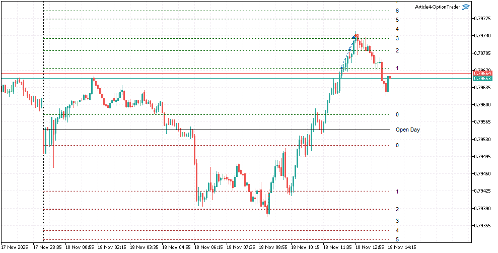
Fig. 2. Level-based expiration of a Long Straddle option structure

It is recommended to determine the level number for expiration based on historical volatility statistics for the underlying asset. In addition, you can use the built-in tester in MetaTrader 5 to determine the optimal expiration level.

Adaptive Calculation of Historical Volatility (HV)

Before moving on, let's refine the algorithm for calculating historical volatility (HV). Instead of specifying a fixed window length in the input parameters, we will select the number of days for the calculation adaptively. By varying the window length from three to forty (the optimization range was selected empirically), we select the window with the minimum average deviation from the actual values.

Let's add parameters to our EA for setting the limits when optimizing the calculation window for historical volatility (HV):

// ---------------------------------------------------------------------
input int  OptimizeDayNumberMin = 3;    // Optimize Minimum Number of Days
input int  OptimizeDayNumberMax = 40;   // Optimize Maximum Number of Days
// ---------------------------------------------------------------------

The minimum and maximum number of completed days are specified, and the optimal window (in terms of error) is sought within this range to calculate the historical volatility (HV).

For our calculations, we will use the standard statistics library included with the MetaTrader 5 platform. For each window length, we perform the following sequence of calculations:

1. Calculate the median HV value for the current window wnd — this gives us the value MedianHV(wnd).
2. We compute an array of absolute differences between the median value obtained in the previous step MedianHV(wnd) and the actual daily range for each day in the array of underlying asset prices — this gives us an array of errors (in absolute value) Error[i] = |HV[i] - MedianHV(wnd)|.
3. We calculate the median value in the resulting array of errors — this gives us the HV estimation error for this window length relative to the actual values — MedianErr = Median(Error[]).

Repeat the calculations from steps 1–3 for each window wnd in the specified optimization range and obtain an array of errors MedianErr[]. The minimum error will correspond to the optimal window for the current day among those calculated from prior volatility values. We will use that window to calculate HV.

NOTE:

We use medians to exclude extremely high and extremely low historical volatility values from our calculations. This will reduce the impact of the "fat tails" of the actual distribution of price increments on the calculation of the HV value.

The complete code for the adaptive calculation of historical volatility (HV) is located in the file HistoryVolatilityA4.mqh, included with this article. Consider the main part of the code shown below:

#include  <Object.mqh>
#include  <Arrays\List.mqh>
// ---------------------------------------------------------------------
#include  <Math\Stat\Stat.mqh>
// --------------------------------------------------------------------

// =====================================================================
//  Calculate the average daily range (ADR):
// =====================================================================
class ResultVolatility : public CObject
{
private:
  int     days_number;
  double  volatility_error;
  double  volatility;

public:
  // --------------------------------------------------------------------
  //  Constructor:
  // --------------------------------------------------------------------
  ResultVolatility(const int _days_number, const double _volatility_error, const double _volatility)
  :
  days_number(_days_number),
  volatility_error(_volatility_error),
  volatility(_volatility),
  CObject()
  {
  }
  // --------------------------------------------------------------------
  int     DaysNumber()
  {
    return(this.days_number);
  }
  // --------------------------------------------------------------------
  double  VolatilityError()
  {
    return(this.volatility_error);
  }
  // --------------------------------------------------------------------
  double  Volatility()
  {
    return(this.volatility);
  }
};
// --------------------------------------------------------------------
class TDailyVolatility
{
protected:
  string    data_symbol;
  datetime  data_start_time;
  datetime  data_end_time;

  int       min_days_number;
  int       max_days_number;

  MqlRates  daily_data_rates_Array[ ];
  double    daily_range_Array[];
  double    daily_errors_Array[];
  CList*    results_List;

  int       optimal_days_number;
  double    optimal_volatility;
  double    optimal_volatility_error;

  bool      data_prepared_flag;
  bool      volatility_calculated_flag;

public:
  // --------------------------------------------------------------------
  //  Constructor:
  // --------------------------------------------------------------------
  TDailyVolatility(const string _symbol, const int _min_days, const int _max_days)
  :
  data_symbol(_symbol),
  min_days_number(_min_days),
  max_days_number(_max_days),
  data_prepared_flag(false),
  volatility_calculated_flag(false)
  {
    this.results_List = new CList();
    this.results_List.FreeMode(true);
  }

protected:
  // ---------------------------------------------------------------------
  //  Retrieve time series data within a specified time range:
  // ---------------------------------------------------------------------
  bool  PrepareData(const datetime _start_time, const int _days_number)
  {
    if(CopyRates(this.data_symbol, PERIOD_D1, _start_time, _days_number, this.daily_data_rates_Array) <= 0)
    {
      this.data_prepared_flag = false;
    }
    else
    {
      this.data_prepared_flag = true;
      this.data_start_time = this.daily_data_rates_Array[0].time;
      this.data_end_time = this.daily_data_rates_Array[ArraySize(this.daily_data_rates_Array) - 1].time;
    }
   
    return(this.data_prepared_flag);
  }

protected:
  // ---------------------------------------------------------------------
  //  Daily volatility for the specified range of days:
  // ---------------------------------------------------------------------
  bool  CalcDayRange(const int _day_start_index, const int _days_number)
  {
    if(this.data_prepared_flag != true)
    {
      return(false);
    }

    int   max_day_index = MathMin(_days_number, ArraySize(this.daily_data_rates_Array));
    ArrayResize(this.daily_range_Array, _days_number);

    for(int i = 0; i < max_day_index; i++)
    {
      this.daily_range_Array[i] = this.daily_data_rates_Array[i + _day_start_index].high - this.daily_data_rates_Array[i + _day_start_index].low;
    }

    return(true);
  }
  // ---------------------------------------------------------------------

public:
  // ---------------------------------------------------------------------
  //  ADR calculation:
  // ---------------------------------------------------------------------
  bool  CalculateADR(const datetime _current_time)
  {
    this.volatility_calculated_flag = false;

    //  Obtain the time series data:
    if(this.PrepareData(_current_time, max_days_number - min_days_number + 1) != true)
    {
      return(false);
    }

    ArrayResize(daily_errors_Array, max_days_number - min_days_number + 1);
    if(CalcDayRange(0, max_days_number - min_days_number + 1) != true)
    {
      return(false);
    }

    double  curr_volatitlity_Arr[];
    double  curr_volatitlity_error_Arr[];
    double  curr_median_volatility;
    double  curr_median_volatility_error;

    this.results_List.Clear();
    for(int wnd_length = min_days_number; wnd_length < max_days_number; wnd_length++)
    {
      ArrayResize(curr_volatitlity_Arr, wnd_length);
      ArrayResize(curr_volatitlity_error_Arr, wnd_length);

      ArrayCopy(curr_volatitlity_Arr, this.daily_range_Array, 0, max_days_number - min_days_number - wnd_length, wnd_length);

      curr_median_volatility = MathMedian(curr_volatitlity_Arr);
      for(int i = 0; i < wnd_length; i++)
      {
        curr_volatitlity_error_Arr[i] = MathAbs(curr_volatitlity_Arr[i] - curr_median_volatility);
      }
      curr_median_volatility_error = MathMedian(curr_volatitlity_error_Arr);
      this.results_List.Add(new ResultVolatility(wnd_length, curr_median_volatility_error, curr_median_volatility));
    }

    if(this.results_List.Total() <= 0)
    {
      return(false);
    }

    this.optimal_volatility_error = DBL_MAX;

    ResultVolatility* curr_result = this.results_List.GetFirstNode();
    while(true)
    {
      if(curr_result.VolatilityError() < this.optimal_volatility_error)
      {
        this.optimal_days_number = curr_result.DaysNumber();
        this.optimal_volatility_error = curr_result.VolatilityError();
        this.optimal_volatility = curr_result.Volatility();
      }
      curr_result = this.results_List.GetNextNode();
      if(CheckPointer(curr_result) == POINTER_INVALID)
      {
        break;
      }
    }
  
    this.volatility_calculated_flag = true;
    return(true);
  }
};

The ResultVolatility class, used to store results, is derived from the CObject class from the standard library of the MetaTrader 5. This is done so that the standard CList list class can be used to manipulate the results. An object of the ResultVolatility class contains the calculation results for one step (one window value) of the adaptive volatility calculation. These are data members with the following values: window length, volatility calculation error, and calculated volatility.

The constructor of the volatility calculation class TDailyVolatility(const string symbol, const int min_days, const int max_days) accepts the following values as arguments:

• symbol — the name of the working symbol (may differ from the chart symbol on which the EA is installed,
• min_days — the minimum window size used in optimization when calculating historical volatility (HV) (the default value is three),
• max_days — the maximum window size used in optimization when calculating historical volatility (HV) (the default value is 40).

The main method called for calculating historical volatility (HV):

bool  CalculateADR(const datetime _current_time)

The current time is passed as an argument — for example, the opening time of a new bar on the chart on which the EA is installed. This method performs the entire adaptive historical volatility calculation sequence: it loads a time series of historical data, calculates daily volatility values, the median value, and the optimal window.

After successfully calling the method TDailyVolatility::CalculateADR (in this case, it returns true), you can retrieve the calculated optimal parameters using simple methods:

double  GetOptimalVolatility();    // retrieve the calculated volatility
double  GetOptimalVolatilityVar(); // retrieve the calculated volatility error
int     GetOptimalDaysNumber();    // retrieve the calculated value of the optimal window — the number of days

In the EA, volatility is recalculated once a day at the start of a new day and when the EA is restarted during the current, incomplete day. After the calculation, the option levels and their display on the chart are updated.

Risk Management for Strategies Based on Written Options

As shown in the previous article, option strategies based on written options carry unlimited risk. It turns out there is a way to limit this risk by making the option structure more complex. This can be done by adding two more options to the option structure — a Long Put and a Long Call.

The strike prices of these options must lie beyond the maximum option levels in both the positive and negative DPrice regions (see Fig. 7 in the previous article). In that case, the resulting graph showing the relationship between the PnL (profit/loss) value and the relative price change, DPrice, will take the form shown in Figs. 5 and 7.

As can be seen in the figures, the resulting graph has distinctive bends to the right and left of zero; this payoff shape is called a "butterfly" (or "condor," depending on whether the graph is oriented upward or downward). In English, we will refer to this structure as Butterfly — we will add this word to the end of the general name of the option structure.

If we look at the graph showing the relationship between the delta of an option structure (Delta) and the relative price change (DPrice) in Fig. 4, we can see that after reaching a peak with a delta value of approximately one (or minus one), the delta curve on the graph moves toward zero. This is the effect of the long Put/Call options with the appropriate settings.

Thus, the positions are closed out gradually, and if the underlying asset continues to move in a direction that is unfavorable to us, our losses do not increase. When the price reverses from the loss-making region back into the working range defined by HV volatility, the option position is restored to its initial level in accordance with the delta change curve.

We select the normalizing prices and strike prices for these additional Long Put / Long Call options based on acceptable risk. We will set these values (strike price and normalizing level) in the Expert Advisor (EA)'s external parameters. Between the strike price and the normalizing price in the “Butterfly zone” (“Butterfly working area” in Figs. 5 and 7), the option position will be gradually reduced until it is completely closed out. This limits the maximum risk. We will also add the "Butterfly zone" to our EA's level visualizer.

An actual chart showing the option levels is shown in Fig. 3. The option parameters for the "Butterfly zone" are set so that positions are closed out at approximately one quarter of the HV range. This makes it possible to balance the risk/reward ratio for these or similar option structures.

Let's add the following new strategies to our list of option structures:

// ---------------------------------------------------------------------
//  Option structure:
// ---------------------------------------------------------------------
enum ENUM_OPTION_CONSTRUCTION
{
  ENUM_OPTION_CONSTRUCTION_STRADDLE_BUTTERFLY_SHORT = 10,      // Short STRADDLE + Butterfly
  ENUM_OPTION_CONSTRUCTION_STRANGLE_BUTTERFLY_SHORT = 12,      // Short STRANGLE + Butterfly
};
// ---------------------------------------------------------------------

To calculate option levels in the "Short Straddle/Strangle zone," you can use the same methods as in the Short Straddle/Strangle strategy described in the previous article. Since the function relating the delta value "Delta" to the relative price change "DPrice" is no longer monotonic, we will need to divide the function’s domain into two segments in order to correctly calculate option levels across the entire rebalancing range of the option structure: the working region and the “Butterfly zone.” Accordingly, we will add separate calculation methods for these two sections:

void CalculateUpPriceLevels(const double _norm_zero_level, double& _strike_price[], double& _norm_price[], double& _limit_price[]) override
void CalculateDnPriceLevels(const double _norm_zero_level, double& _strike_price[], double& _norm_price[], double& _limit_price[]) override
void CalculateButterflyUpPriceLevels(const double _norm_zero_level, double& _strike_price[], double& _norm_price[], double& _limit_price[])
void CalculateButterflyDnPriceLevels(const double _norm_zero_level, double& _strike_price[], double& _norm_price[], double& _limit_price[])

The first two methods are completely analogous to the methods for the Short Straddle / Short Strangle option structure, while the third and fourth methods have been added to calculate option levels in the “Butterfly zone.” They are declared in descendant classes derived from the base option-structure class: ShortStraddleButterflyOptionConstruction and ShortStrangleButterflyOptionConstruction. The calculation algorithm for the last two methods is identical: it is the bisection method, also known as the method of dichotomy.

We will also add external parameters to configure the visualization of the option levels in the "Butterfly zone":

// ---------------------------------------------------------------------
input color     OptionButterflyUpLevelsTextColor = clrLightYellow;    // Option Butterfly Up Levels Text Color
input color     OptionButterflyUpLevelsColor = clrGreen;              // Option Butterfly Up Levels Color
input ENUM_LINE_STYLE OptionButterflyUpLevelsStyle = STYLE_DOT;       // Option Butterfly Up Levels Line Style
// ---------------------------------------------------------------------
input color     OptionButterflyDnLevelsTextColor = clrLightYellow;    // Option Butterfly Dn Levels Text Color
input color     OptionButterflyDnLevelsColor = clrRed;                // Option Butterfly Dn Levels Color
input ENUM_LINE_STYLE OptionButterflyDnLevelsStyle = STYLE_DOT;       // Option Butterfly Dn Levels Line Style
// ---------------------------------------------------------------------

An example visualization of the calculated levels for the Short Strangle Butterfly option structure is shown below in Fig. 3. The left half shows the upper (above the opening price) option levels, while the right half shows the lower (below the opening price) option levels. The levels of the working region and the "Butterfly zone" have been calculated for the values specified below.

input double    StrangleKoeffStrike = 0.1;                            // Strangle Coefficient for Strike (0.01...0.90)
input double    ButterflyKoeffStrike = 0.94;                          // Butterfly Coefficient for Strike (0.60...2.00)
input double    ButterflyKoeffNorm = 1.345;                           // Butterfly Coefficient for Strike (1.00...2.00)

The value of the ButterflyKoeffStrike parameter sets the strike price position for the Butterfly zone; this is the strike price for the Long Put and Long Call options. It is specified as a coefficient by which the historical volatility (HV) value is multiplied. In this zone, the deltas of the Short Put and Short Call options are equal to plus or minus one and no longer change as the price of the underlying asset continues to rise or fall. By contrast, the delta of the options in the Butterfly zone moves away from zero and begins to reduce the total value of the option position as the price of the underlying asset continues to rise or fall, eventually bringing it down to zero.

The lower the value of the ButterflyKoeffStrike parameter, the sooner the size of the option position starts to decrease.

The value of the ButterflyKoeffNorm parameter sets the HV-based normalizing level for the Long Put and Long Call options. It is also specified as a multiplier by which the historical volatility (HV) value for the current day is multiplied. Increasing the value of ButterflyKoeffNorm expands the Butterfly zone within which the option position is closed, meaning that the close-out becomes smoother.

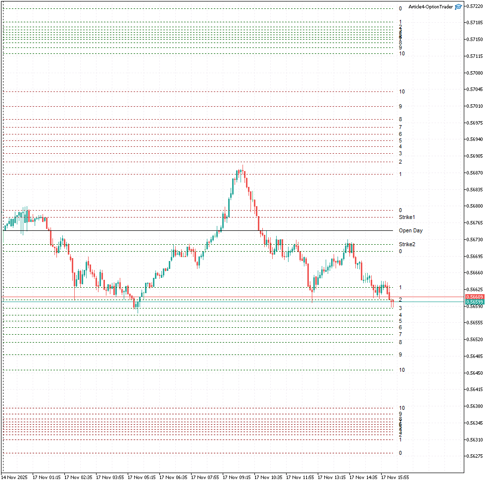
Fig. 3. Option levels calculated for the Short Strangle Butterfly option structure.

Let's examine the rationale and conditions for using the Butterfly structures listed above.

Selling a straddle with a “Butterfly” — Short Straddle Butterfly

• Rationale: the simultaneous sale of call and put options with the same strike prices;
• Condition for use: if you are confident that the price of the underlying asset will remain within the average historical volatility (HV) range, and the direction of its movement does not matter;
• Profit: the premium paid by the buyer for the two options (absent in emulation) + the profit accumulated when the price fluctuates within the range (available only in emulation);
• Risk: limited by the parameters of the “Butterfly” options.

Using a straddle with a "Butterfly" is similar to using a simple straddle, as described in the previous article. An example of how the Short Straddle Butterfly option structure works is shown in Fig. 6.

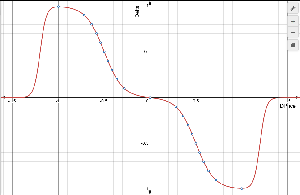
Fig. 4. Dependence of the "Delta" value on the relative price change "DPrice" for the emulated Short Straddle Butterfly option structure

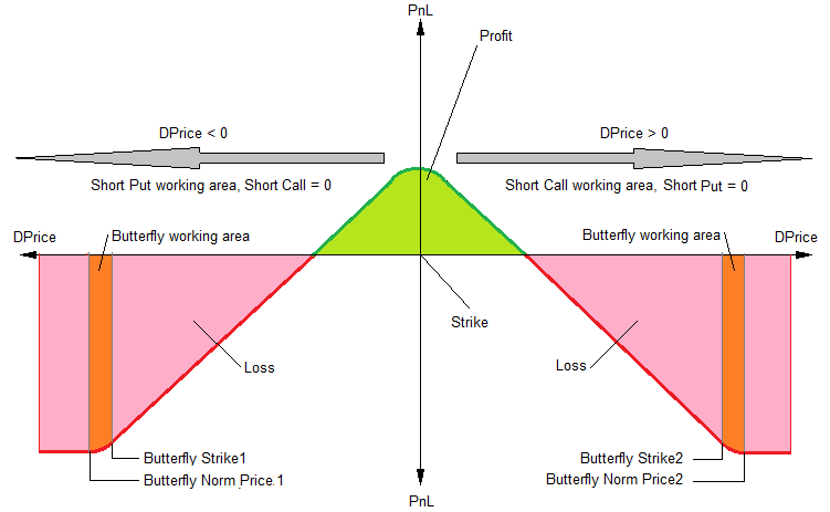
Fig. 5. Dependence of the PnL (profit/loss) value on the relative price change "DPrice" for the emulated Short Straddle Butterfly option structure

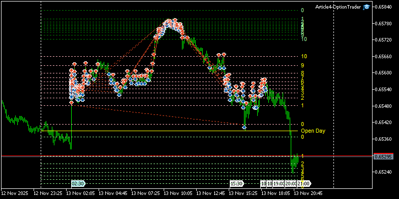
Fig. 6. Example of how a Short Straddle Butterfly option structure works

Selling a Strangle — Short Strangle Butterfly

• Rationale: simultaneously writing call and put options with different strike prices that lie within the historical volatility (HV) range;
• Condition for use: if you are confident that the price of the underlying asset will remain within a wide range, and its direction is irrelevant;
• Profit: the premium the buyer pays for the two options (absent in emulation) + the profit accumulated as the price fluctuates within a wide range;
• Risk: limited by the parameters of the “butterfly” options.

Using a strangle with a “butterfly” is similar to using a simple strangle, as described in the previous article. An example of how the Short Strangle Butterfly option structure works is shown in Fig. 8. In this case, the price did not continue to fall, but we prevented a potential large loss.

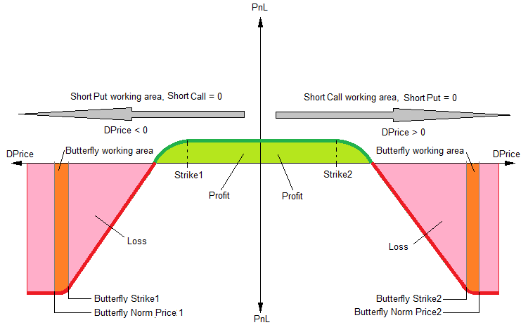
Fig. 7. Dependence of the PnL (profit/loss) value on the relative price change “DPrice” for the emulated Short Strangle Butterfly option structure

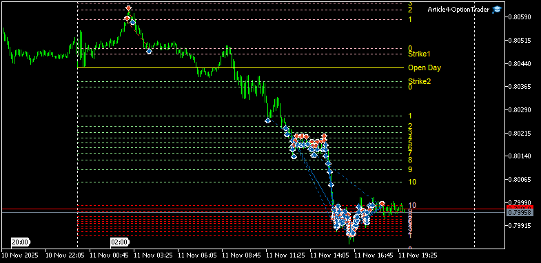
Fig. 8. Example of how a Short Strangle Butterfly option structure works

It is best to select the “butterfly” parameters for option-writing strategies based on the results of a statistical analysis of the historical volatility of the underlying asset. We determine the magnitude and frequency of “fat tails,” then test the strategy using MetaTrader 5’s built-in tester to minimize losses in these areas, thereby optimizing the “butterfly” parameters.

Conclusion

In this article, we explored possible ways to reduce risk and increase profitability for complex option strategies. In the next article in this series, we'll look at a few more practical applications of options. In particular, we will consider trading synthetic instruments. We will also add new features to our Expert Advisor (EA) — trading on netting accounts, interactive control of certain parameters, and more.

In addition, we will conduct some statistical studies to determine the optimal trading parameters.

NOTE:

It is also important to understand that trading options (as with other instruments) requires the trader’s involvement at every stage of implementing a strategy — from developing a money management system to monitoring trades in real time.

The table lists the files attached to the article:

File name	Description
Article4-OptionTrader.mq5	Code for the Expert Advisor (EA) that trades the option structures described in the article using option emulation
CheckNewBar.mqh	Code for the class that checks for a new bar on a MetaTrader 5 chart
OptionEmulatorA4.mqh	Code for the classes used to emulate the options and option structures described in the article
PriceLevelsA4.mqh	Code for the classes used to visualize option levels on a MetaTrader 5 chart
HistoryVolatilityA4.mqh	Code for the classes used for adaptive calculation of historical volatility (HV)