
Neural Networks in Trading: Anomaly Detection in the Frequency Domain (Final Part)

Introduction
In the previous article, we introduced the innovative CATCH framework for anomaly detection in multivariate time series. The frequency-domain analysis method proposed by the framework's authors enables not only the detection of point anomalies such as outliers and abrupt changes, but also the identification of more complex hidden patterns that often evade traditional approaches. The CATCH framework employs the Fourier transform to convert data from the time domain into its spectral representation, opening new opportunities for a detailed analysis of the characteristics of the sequence under examination.
One of the key advantages of CATCH is its use of frequency patching. Instead of analyzing the entire spectrum as a whole, the model divides it into separate fragments corresponding to specific frequency ranges. This approach makes it possible to examine both global trends and local features associated with high-frequency components. As a result, various types of anomalies can be identified and classified with high precision, whether they are short-term spikes or more complex deviations at the subsequence level. Such spectral partitioning enables a much more detailed study of the time-series structure.
An important component of the framework is the adaptive module responsible for analyzing relationships between different data channels. This component, which implements a masked attention mechanism, allows the system to focus on the most significant correlations while filtering out noise and irrelevant information. This mechanism improves the reconstruction quality of normal behavior and significantly enhances model robustness in a changing market environment. Unlike traditional methods that process channels independently, CATCH takes their complex interdependencies into account. This is particularly important when working with financial data, where movements in one market can influence other segments.
At the final stage of the CATCH framework, the original time series is reconstructed. After detailed frequency-domain analysis and the identification of potential anomalies, the system performs an inverse transformation, returning the data to its conventional time-domain representation. The difference between the original values and the reconstructed time series serves as a reliable indicator of deviations, enabling a timely response to changes in market dynamics.
The authors' visualization of the CATCH framework is shown below.

In the practical section of the previous article, we began implementing our own interpretation of the proposed approaches using MQL5. Specifically, we developed a convolutional layer for processing complex-valued data. We also examined the implementation of the forward and backward passes of the complex-valued masked attention module within an OpenCL context. Today, we continue this work.
Complex-Valued Masked Attention Object
In the previous article, we examined the MaskAttentionComplex and MaskAttentionGradientsComplex kernels, which implement the forward and backward propagation algorithms of the masked attention mechanism in the complex domain. Today, we continue this work. We will organize the masked attention module on the main application side. To achieve this, we create a new object CNeuronComplexMVMHMaskAttention having the following structure:
class CNeuronComplexMVMHMaskAttention :  public CNeuronBaseOCL
  {
protected:
   uint                       iWindow;
   uint                       iWindowKey;
   uint                       iHeads;
   uint                       iUnits;
   uint                       iVariables;
   //---
   CNeuronComplexConvOCL      cQKV;
   CNeuronBaseOCL             cQ;
   CNeuronBaseOCL             cKV;
   CNeuronConvOCL             cMask;
   CNeuronBaseOCL             cMHAttentionOut;
   CNeuronComplexConvOCL      cPooling;
   CNeuronBaseOCL             cResidual;
   CNeuronComplexConvOCL      cFeedForward[2];
   //---
   virtual bool               AttentionOut(void);
   virtual bool               AttentionInsideGradients(void);
   virtual bool               SumAndNormilize(CBufferFloat *tensor1, CBufferFloat *tensor2, CBufferFloat *out,
                                              int dimension, bool normilize = true, int shift_in1 = 0,
                                              int shift_in2 = 0, int shift_out = 0, float multiplyer = 0.5f) override;
   //---
   virtual bool               feedForward(CNeuronBaseOCL *NeuronOCL) override;
   virtual bool               updateInputWeights(CNeuronBaseOCL *NeuronOCL) override;
   virtual bool               calcInputGradients(CNeuronBaseOCL *prevLayer) override;

public:
                     CNeuronComplexMVMHMaskAttention(void) {};
                    ~CNeuronComplexMVMHMaskAttention(void) {};
   //---
   virtual bool               Init(uint numOutputs, uint myIndex, COpenCLMy *open_cl,
                                   uint window, uint window_key, uint heads,
                                   uint units_count, uint variables,
                                   ENUM_OPTIMIZATION optimization_type, uint batch);
   //---
   virtual int                Type(void)   const   {  return defNeuronComplexMVMHMaskAttention;   }
   //---
   virtual bool               Save(int const file_handle) override;
   virtual bool               Load(int const file_handle) override;
   //---
   virtual bool               WeightsUpdate(CNeuronBaseOCL *source, float tau) override;
   virtual void               SetOpenCL(COpenCLMy *obj) override;
  };
As can be seen, the structure of this new object is fairly standard for attention modules, several variations of which have already been implemented in our library. However, there is one important distinction associated with the use of complex-valued data. The object is designed to receive input data that has already been converted into complex form, allowing us to omit the data transformation stage. To generate the Query, Key, and Value representations, we use the previously developed convolutional layer for complex-valued processing. Let us examine the implementation step by step.
All internal objects are declared as class members, allowing us to keep the class constructor and destructor empty. The initialization of these declared and inherited objects is performed in the Init method. This method receives a set of constants that uniquely define the architecture of the object being created. Their structure is fairly typical for such objects.
bool CNeuronComplexMVMHMaskAttention::Init(uint numOutputs, uint myIndex, COpenCLMy *open_cl,
                                           uint window, uint window_key, uint heads,
                                           uint units_count, uint variables,
                                           ENUM_OPTIMIZATION optimization_type, uint batch)
  {
//---
   if(!CNeuronBaseOCL::Init(numOutputs, myIndex, open_cl, 2 * window * units_count * variables,
                                                                      optimization_type, batch))
      return false;
At the beginning of the method, we call the corresponding method of the parent class, which already contains the initialization logic for inherited objects and interfaces. We then store the model architecture parameters received from the external program in internal variables.
   iWindow = window;
   iWindowKey = MathMax(window_key, 1);
   iUnits = units_count;
   iHeads = MathMax(heads, 1);
   iVariables = variables;
Next, we proceed with the initialization of the newly declared objects. The first component to be initialized is the mask generation module.
It is worth noting that the framework's authors propose a mask generation module based on a trainable projection of the input data. In addition, a multi-head attention mechanism is used, with each attention head using its own unique mask.
Another important aspect is that attention is not applied across the entire frequency spectrum. The CATCH framework applies attention only within individual patches corresponding to the same frequency segment but belonging to different univariate sequences.
Naturally, the output of the mask generation module must be a probabilistic representation of the influence of individual channels in the form of real-valued coefficients.
To satisfy these requirements, our implementation employs a standard convolutional layer with a doubled kernel size (to accommodate complex-valued windows) and a number of filters equal to the dimensionality of the masking vector for a single sequence element.
   uint index = 0;
   if(!cMask.Init(0, index, OpenCL, 2 * iWindow, 2 * iWindow, iVariables * iHeads,
                                         iUnits, iVariables, optimization, iBatch))
      return false;
   cMask.SetActivationFunction(SIGMOID);
   CBufferFloat *temp = cMask.GetWeightsConv();
   if(!temp ||
      !temp.Fill(0))
      return false;
To ensure that the output values remain within the required range, we use a sigmoid activation function.
Note that during initialization, the trainable parameter matrix is filled with zeros. This allows all elements to begin with an equal influence mask value of 0.5. During training, the weights will be adjusted, gradually modifying the dependency mask between channels.
Next, we initialize the module responsible for generating the Query, Key, and Value representations. Here, we employ a complex-valued convolutional layer, since both the input and output of the module are expected to be complex-valued.
   index++;
   if(!cQKV.Init(0, index, OpenCL, iWindow, iWindow, 3 * iWindowKey * iHeads,
                                    iUnits, iVariables, optimization, iBatch))
      return false;
   cQKV.SetActivationFunction(None);
We then divide the combined tensor containing all three representations into two parts and extract the Query entity into a separate matrix. To support this operation, we initialize two additional objects. The method then completes execution, returning a Boolean result indicating whether all operations were performed successfully.
   index++;
   if(!cQ.Init(0, index, OpenCL, 2 * iWindowKey * iHeads * iVariables * iUnits, optimization, iBatch))
      return false;
   cQ.SetActivationFunction(None);
   index++;
   if(!cKV.Init(0, index, OpenCL, 2 * cQ.Neurons(), optimization, iBatch))
      return false;
   cKV.SetActivationFunction(None);
At the same stage, we initialize the object responsible for storing the multi-head attention results.
   index++;
   if(!cMHAttentionOut.Init(0, index, OpenCL, cQ.Neurons(), optimization, iBatch))
      return false;
   cMHAttentionOut.SetActivationFunction(None);
We then add a complex-valued convolutional layer for reducing the dimensionality of the attention outputs.
   index++;
   if(!cPooling.Init(0, index, OpenCL, iWindowKey * iHeads, iWindowKey * iHeads,
                              iWindow, iUnits, iVariables, optimization, iBatch))
      return false;
   cPooling.SetActivationFunction(None);
Similar to the classical Transformer architecture, we add a layer to preserve residual connections.
   index++;
   if(!cResidual.Init(0, index, OpenCL, cPooling.Neurons(), optimization, iBatch))
      return false;
   cResidual.SetActivationFunction(None);
This is followed by two complex-valued convolutional layers of the FeedForward module.
   index++;
   if(!cFeedForward[0].Init(0, index, OpenCL, iWindow, iWindow, 4 * iWindow,
                                  iUnits, iVariables, optimization, iBatch))
      return false;
   cFeedForward[0].SetActivationFunction(LReLU);
   index++;
   if(!cFeedForward[1].Init(0, index, OpenCL, 4 * iWindow, 4 * iWindow, iWindow,
                                       iUnits, iVariables, optimization, iBatch))
      return false;
   cFeedForward[1].SetActivationFunction(None);
   SetActivationFunction(None);
//---
   return true;
  }
Finally, we complete the object initialization procedure, returning a Boolean result indicating the success of the operation to the calling program.
The next step is to construct the forward propagation algorithm within the feedForward method.
bool CNeuronComplexMVMHMaskAttention::feedForward(CNeuronBaseOCL *NeuronOCL)
  {
   if(!NeuronOCL)
      return false;
The method receives a pointer to the input data object, whose validity is verified immediately.
To improve training stability, the input data is normalized.
   if(!NeuronOCL.SwapOutputs())
      return false;
   if(!SumAndNormilize(NeuronOCL.getPrevOutput(), NeuronOCL.getPrevOutput(), NeuronOCL.getOutput(),
                       iWindow, true, 0, 0, 0, 1))
      return false;
It should be noted that the input data consists of complex-valued quantities. Therefore, the summation and normalization methods were redefined to support complex-valued operations. The complete implementation can be found in the attached source code.
After normalization, the input data is used to generate the masking tensors and the Query, Key, and Value entities.
   if(!cMask.FeedForward(NeuronOCL))
      return false;
   if(!cQKV.FeedForward(NeuronOCL))
      return false;
We then split the combined tensor of generated entities into two separate tensors.
   if(!NeuronOCL.SwapOutputs())
      return false;
   if(!DeConcat(cQ.getOutput(), cKV.getOutput(), cQKV.getOutput(), 2 * iWindowKey * iHeads,
                                              4 * iWindowKey * iHeads, iUnits * iVariables))
      return false;
All prepared data is subsequently passed to the masked attention forward-pass kernel. This operation is performed within a dedicated method named AttentionOut.
   if(!AttentionOut())
      return false;
We then reduce the dimensionality of the resulting multi-head attention output and sum the output with the original input data to establish residual connections.
   if(!cPooling.FeedForward(cMHAttentionOut.AsObject()))
      return false;
   if(!SumAndNormilize(NeuronOCL.getOutput(), cPooling.getOutput(), cResidual.getOutput(), iWindow, true, 0, 0, 0, 1))
      return false;
The data is subsequently passed through the two convolutional layers of the FeedForward module.
   if(!cFeedForward[0].FeedForward(cResidual.AsObject()))
      return false;
   if(!cFeedForward[1].FeedForward(cFeedForward[0].AsObject()))
      return false;
Again we add residual connections. We save the final output in the inherited buffer used for data exchange with other neural layers of the model.
   if(!SumAndNormilize(cResidual.getOutput(), cFeedForward[1].getOutput(), getOutput(), iWindow, true, 0, 0, 0, 1))
      return false;
//---
   return true;
  }
The method concludes by returning the logical result of the operation to the calling program.
A few words should be said about the AttentionOut method, which is responsible for enqueuing the execution of the multi-head masked attention kernel MaskAttentionComplex. In recent work, we have rarely discussed the mechanics of submitting OpenCL kernels to the execution queue. This is understandable. The procedure for enqueuing kernels is fairly standard. And there is no need to repeatedly describe the same operations. However, in this case, there is an important nuance related to the CATCH framework.
As mentioned above, the authors of the CATCH framework propose performing masked attention strictly between elements within the same frequency range across different univariate sequences. In simple terms, we take identical frequency patches from different univariate sequences and analyze their interdependencies. This allows us to independently identify relationships within different univariate sequences across frequency bands—separately capturing long-term trends and short-term dynamics. However, this property was not explicitly accounted for when designing a unified masked attention kernel.
Nevertheless, we can still organize the required behavior by controlling the task space used for the kernel execution queue. To begin with, let us examine the dimensionality of the input data received by the object. We are working with segmented data from a multivariate sequence, which can be represented as a three-dimensional tensor: {Variable, Segment, Dimension}. Further, when constructing entities for multi-head attention, each output can be represented as a four-dimensional tensor: {Variable, Segment, Head, Dimension}.
It is important to note that our multi-head attention implementation processes each attention head independently. Therefore, if we merge the segment and head dimensions and treat each segment as an independent attention head, we effectively obtain an analysis of dependencies between identical segments across different univariate sequences. This is precisely the behavior required to correctly implement the CATCH framework.
The AttentionOut method does not take any parameters. In the method's control block, we only verify the validity of the pointer to the OpenCL context management object.
bool CNeuronComplexMVMHMaskAttention::AttentionOut(void)
  {
   if(!OpenCL)
      return false;
Next, we define arrays describing the kernel execution space. As discussed earlier, the sequence dimension is set to the number of univariate sequences in the dataset. For the number of heads, we use the product of the configured number of attention heads and the number of segments in each sequence.
   uint global_work_offset[3] = {0};
   uint global_work_size[3] = {iVariables/*Q units*/, iVariables/*K units*/, iHeads * iUnits/*Heads*/};
   uint local_work_size[3] = {1, iVariables, 1};
We then group execution threads into work-groups along the second dimension of the task space.
After that, we pass pointers to the required data buffers as kernel arguments.
   ResetLastError();
   int kernel = def_k_MaskAttentionComplex;
   if(!OpenCL.SetArgumentBuffer(kernel, def_k_maskattcom_q, cQ.getOutputIndex()))
     {
      printf("Error of set parameter kernel %s: %d; line %d", __FUNCTION__, GetLastError(), __LINE__);
      return false;
     }
   if(!OpenCL.SetArgumentBuffer(kernel, def_k_maskattcom_kv, cKV.getOutputIndex()))
     {
      printf("Error of set parameter kernel %s: %d; line %d", __FUNCTION__, GetLastError(), __LINE__);
      return false;
     }
   if(!OpenCL.SetArgumentBuffer(kernel, def_k_maskattcom_scores, cMask.getPrevOutIndex()))
     {
      printf("Error of set parameter kernel %s: %d; line %d", __FUNCTION__, GetLastError(), __LINE__);
      return false;
     }
   if(!OpenCL.SetArgumentBuffer(kernel, def_k_maskattcom_out, cMHAttentionOut.getOutputIndex()))
     {
      printf("Error of set parameter kernel %s: %d; line %d", __FUNCTION__, GetLastError(), __LINE__);
      return false;
     }
   if(!OpenCL.SetArgumentBuffer(kernel, def_k_maskattcom_masks, cMask.getOutputIndex()))
     {
      printf("Error of set parameter kernel %s: %d; line %d", __FUNCTION__, GetLastError(), __LINE__);
      return false;
     }
At this point, we take advantage of the fact that the attention coefficient matrix shares the same dimensionality as the channel masking matrix. This allows us to avoid allocating an additional buffer for temporary storage of attention coefficients. Instead, an unused buffer from the mask generation module is reused for this purpose.
We then pass the remaining necessary parameters to the kernel.
   if(!OpenCL.SetArgument(kernel, def_k_maskattcom_dimension, (int)iWindowKey))
     {
      printf("Error of set parameter kernel %s: %d; line %d", __FUNCTION__, GetLastError(), __LINE__);
      return false;
     }
   if(!OpenCL.SetArgument(kernel, def_k_maskattcom_heads_kv, (int)(iHeads * iUnits)))
     {
      printf("Error of set parameter kernel %s: %d; line %d", __FUNCTION__, GetLastError(), __LINE__);
      return false;
     }
It is also worth noting that, for both Key and Value representations, we again define the number of attention heads as the product of the user-defined head count and the sequence length.
Finally, we enqueue the kernel for execution.
   if(!OpenCL.Execute(kernel, 3, global_work_offset, global_work_size, local_work_size))
     {
      printf("Error of execution kernel %s: %d", __FUNCTION__, GetLastError());
      return false;
     }
//---
   return true;
  }
The method ends by returning a logical result to the calling program.
After completing the forward-pass algorithms, we proceed to the construction of the backpropagation procedures. The first step is to implement the method responsible for distributing the error gradients across all internal components according to their contribution to the final model output: calcInputGradients.
bool CNeuronComplexMVMHMaskAttention::calcInputGradients(CNeuronBaseOCL *prevLayer)
  {
   if(!prevLayer)
      return false;
The method receives the same input data object used during the feed-forward pass. However, this time it is used to propagate the corresponding error gradients. We immediately verify the pointer validity.
At this stage, the external interface buffer of the object contains the error gradient received from the subsequent layer. These values have not yet been adjusted by the derivative of the activation function. This is intentional: the activation function was deliberately omitted during initialization. This is done to provide flexibility in selecting activation functions for internal objects. We now apply the derivative of the activation function of the final convolutional layer in the FeedForward module and propagate the corrected gradients accordingly.
   if(!DeActivation(cFeedForward[1].getOutput(), cFeedForward[1].getGradient(), Gradient, cFeedForward[1].Activation()))
      return false;
We then propagate the gradients backward through the layers of the module up to the residual connection level following the attention block.
   if(!cFeedForward[0].calcHiddenGradients(cFeedForward[1].AsObject()))
      return false;
   if(!cResidual.calcHiddenGradients(cFeedForward[0].AsObject()))
      return false;
For the residual connection object, we also assume the absence of an activation function. We therefore repeat the gradient correction procedure using the derivative of the activation function applied to the attention output scaling layer.
   if(!DeActivation(cPooling.getOutput(), cPooling.getGradient(), cResidual.getGradient(), cPooling.Activation()) ||
      !DeActivation(cPooling.getOutput(), cPooling.getPrevOutput(), Gradient, cPooling.Activation()) ||
      !SumAndNormilize(cPooling.getGradient(), cPooling.getPrevOutput(), cPooling.getGradient(), iWindow,
                                                                                       false, 0, 0, 0, 1))
      return false;
However, it is important to emphasize that the residual connection object currently contains only the gradient flowing through the FeedForward path. We must also account for the gradient flowing through the residual attention path. Therefore, we again correct the gradient stored in the external interface buffer using the derivative of the activation function of the attention output projection layer.
It should be noted that reusing the external interface buffer does not imply double transformation of the data. In the first case, the corrected values were stored in the buffer of the final FeedForward layer, while the interface buffer itself retained the original gradient values. In the current step, the computations are written into the projection layer buffer without modifying the original data, which will later be reused when propagating gradients through the residual connection back to the input level.
After these corrections, we sum the contributions from both information flows. The gradient is then distributed across the attention heads.
   if(!cMHAttentionOut.calcHiddenGradients(cPooling.AsObject()))
      return false;
   if(!AttentionInsideGradients())
      return false;
We then call the AttentionInsideGradients method responsible for propagating gradients through the attention mechanism. We will not dwell on the details of this method here. We'll leave it for independent study. Its full implementation is provided in the attachment. However, it should be emphasized that the task space configuration and kernel scheduling parameters must be consistent with those used in the feed-forward pass.
At the next stage, we merge all gradient contributions from the individual attention components into a single tensor.
   if(!Concat(cQ.getGradient(), cKV.getGradient(), cQKV.getGradient(), 2 * iWindowKey * iHeads,
                                                  4 * iWindowKey * iHeads, iUnits * iVariables))
      return false;
We then propagate the error down to the input level, applying the derivative of the corresponding activation function.
   if(!DeActivation(cQKV.getOutput(), cQKV.getPrevOutput(), cQKV.getGradient(), cQKV.Activation()) ||
      !prevLayer.calcHiddenGradients(cQKV.AsObject()))
      return false;
However, this represents only one information flow. We also incorporate the gradient contribution from the residual connection path, applying the derivative of the activation function of the input data processing layer.
In this step, we use data both from the FeedForward module and from the external interface buffer.
   if(!DeActivation(prevLayer.getOutput(),cResidual.getPrevOutput(),cResidual.getGradient(),prevLayer.Activation()) ||
      !SumAndNormilize(prevLayer.getGradient(), cResidual.getPrevOutput(), cResidual.getPrevOutput(),
                       iWindow, false, 0, 0, 0, 1))
      return false;
   if(!DeActivation(prevLayer.getOutput(), cResidual.getGradient(), Gradient, prevLayer.Activation()) ||
      !SumAndNormilize(cResidual.getGradient(), cResidual.getPrevOutput(), cResidual.getPrevOutput(),
                       iWindow, false, 0, 0, 0, 1))
      return false;
It is important to recall that the input data was also used to generate the masking matrix. Therefore, we additionally include the gradient contribution associated with this computation path.
   if(!DeActivation(cMask.getOutput(), cMask.getGradient(), cMask.getGradient(), cMask.Activation()) ||
      !prevLayer.calcHiddenGradients(cMask.AsObject()) ||
      !SumAndNormilize(prevLayer.getGradient(), cResidual.getPrevOutput(), prevLayer.getGradient(),
                       iWindow, false, 0, 0, 0, 1))
      return false;
//---
   return true;
  }
At this point, we have accumulated the full gradient signal across all information flows at the input level, and we can conclude the method by returning a Boolean status to the calling program.
The parameter optimization method is left for independent study. Its logic is relatively straightforward, consisting primarily of calls to the corresponding methods of internal submodules. The full implementation is provided in the attachment, along with the complete code of the object and all its methods. We are moving on to the next stage of our work.
Assembling the CATCH Framework
It can be said that up to this point, a substantial amount of preparatory work has been completed, during which individual objects were developed. Now we proceed to integrate them into a unified structure of the CATCH framework. The execution logic of the framework is implemented within the CNeuronCATCH object, whose structure is shown below.
class CNeuronCATCH   :  public CNeuronTransposeOCL
  {
protected:
   CNeuronTransposeOCL        cTranspose;
   CNeuronBaseOCL             caFreqIn[2];
   CNeuronBaseOCL             cFreqConcat;
   CNeuronComplexConvOCL      caProjection[2];
   CNeuronComplexMVMHMaskAttention  caChannelFusion[2];
   CNeuronComplexConvOCL      caLinearHead[2];
   CNeuronBaseOCL             caFreqOut[2];
   //---
   virtual bool               FFT(CBufferFloat *inp_re, CBufferFloat *inp_im,
                                  CBufferFloat *out_re, CBufferFloat *out_im,
                                  uint variables, bool reverse = false);
   //---
   virtual bool               feedForward(CNeuronBaseOCL *NeuronOCL) override;
   virtual bool               updateInputWeights(CNeuronBaseOCL *NeuronOCL) override;
   virtual bool               calcInputGradients(CNeuronBaseOCL *prevLayer) override;


public:
                     CNeuronCATCH(void) {};
                    ~CNeuronCATCH(void) {};
   //---
   virtual bool               Init(uint numOutputs, uint myIndex, COpenCLMy *open_cl,
                                   uint time_step, uint variables,
                                   uint window, uint step,
                                   uint window_key, uint heads,
                                   ENUM_OPTIMIZATION optimization_type, uint batch);
   //---
   virtual int                Type(void) override const   {  return defNeuronCATCH;   }
   //---
   virtual bool               Save(int const file_handle) override;
   virtual bool               Load(int const file_handle) override;
   //---
   virtual bool               WeightsUpdate(CNeuronBaseOCL *source, float tau) override;
   virtual void               SetOpenCL(COpenCLMy *obj) override;
  };
In the presented structure, we observe a relatively large number of internal components, each responsible for a specific part of the framework's complex processing algorithm. Their roles will be discussed progressively during the implementation of the class methods. For now, it is worth noting that all components are declared statically, which allows both the constructor and destructor to remain empty. The initialization of objects is performed in the Init method.
bool CNeuronCATCH::Init(uint numOutputs, uint myIndex, COpenCLMy *open_cl,
                        uint time_step, uint variables,
                        uint window, uint step, uint window_key, uint heads,
                        ENUM_OPTIMIZATION optimization_type, uint batch)
  {
   if(!CNeuronTransposeOCL::Init(numOutputs, myIndex, open_cl, variables, time_step, optimization_type, batch))
      return false;
The method receives a set of constants that uniquely define the architecture of the initialized object. Some of these parameters define the dimensionality of the input data. Others describe the structure of internal information flows. For example, time_step and variables define the number of time steps and univariate sequences in the multivariate time series. The window and step parameters define the frequency spectrum segmentation strategy. Meanwhile, window_key and heads represent the core parameters of the attention mechanism.
Within the method body, we first call the corresponding method of the parent class. In this case, the parent is a data transposition object, and this choice is intentional. The input is expected to be a multivariate time series represented as a matrix, where each row corresponds to the state vector of the environment at a given time step. However, the CATCH framework operates on the frequency-domain representation of individual univariate sequences. For convenience, we first transpose the input tensor and later restore it to its original representation. The latter operation is performed by the parent class, which is reflected in the parameters passed to it.
To transform the time series into the frequency domain, we use the Fast Fourier Transform. However, this algorithm requires the sequence length to be a power of two. To satisfy this constraint, we can extend any sequence by padding it with zeros, which does not affect the transform result. The next step is to determine the nearest valid sequence length.
//--- Calculate FFT size
   int power = int(MathLog(time_step) / M_LN2);
   if(power <= 0)
      return false;
   if(MathPow(2, power) != time_step)
      power++;
   uint FreqUinits = uint(MathPow(2, power));
We then compute the number of segments according to the specified segmentation parameters.
   if(window <= 0 || step <= 0)
      return false;
   int Segments = int((FreqUinits - int(window) + step - 1) / step);
   if(Segments <= 0)
      return false;
At this point, the preparatory stage is complete, and we proceed to initialize the internal components. The first is the transposition layer for the input data. Its initialization parameters are straightforward and require no special explanation.
   uint index = 0;
   if(!cTranspose.Init(0, index, OpenCL, time_step, variables, optimization, iBatch))
      return false;
Next, we create two data buffers to store the real and imaginary components of the frequency spectrum after Fourier decomposition.
   for(uint i = 0; i < caFreqIn.Size(); i++)
     {
      index++;
      if(!caFreqIn[i].Init(0, index, OpenCL, FreqUinits * variables, optimization, iBatch))
         return false;
      caFreqIn[i].SetActivationFunction(None);
     }
We then add a concatenation module for the frequency-domain representation.
   index++;
   if(!cFreqConcat.Init(0, index, OpenCL, 2 * FreqUinits * variables, optimization, iBatch))
      return false;
   cFreqConcat.SetActivationFunction(None);
For spectral segmentation, we use a complex-valued convolutional layer configured with the appropriate parameters.
   index++;
   if(!caProjection[0].Init(0, index, OpenCL, window, step, 2 * window, Segments, variables, optimization, iBatch))
      return false;
   caProjection[0].SetActivationFunction(LReLU);
A second convolutional layer completes the embedding construction for spectral patches.
   index++;
   if(!caProjection[1].Init(0, index, OpenCL,2*window,2*window,window_key, Segments, variables, optimization, iBatch))
      return false;
   caProjection[1].SetActivationFunction(TANH);
The analysis of interdependencies between frequency spectra of individual univariate sequences is performed using two consecutive attention modules. The first operates directly on the generated patch embeddings.
   index++;
   if(!caChannelFusion[0].Init(0, index, OpenCL,window_key,window_key,heads,Segments, variables, optimization, iBatch))
      return false;
The architecture of the second inter-channel masked attention layer depends on the number of segments. If the number of segments is divisible by two, pairwise merging of segments is performed to capture higher-order dependencies.
   index++;
   if(Segments % 2 == 0)
     {
      if(!caChannelFusion[1].Init(0, index, OpenCL, 2 * window_key, window_key, heads, Segments / 2,
                                                                   variables, optimization, iBatch))
         return false;
     }
   else
      if(!caChannelFusion[1].Init(0, index, OpenCL, window_key, window_key, heads, Segments, variables,
                                                                                 optimization, iBatch))
         return false;
Otherwise, the architecture remains identical to the previous attention layer.
The dimensionality of the tensor produced by the attention modules is then reduced back to the length of the original frequency spectrum using two consecutive projection convolution layers.
   index++;
   if(!caLinearHead[0].Init(0, index, OpenCL, window_key, window_key, window, Segments, variables,
                                                                            optimization, iBatch))
      return false;
   caLinearHead[0].SetActivationFunction(LReLU);
   index++;
   if(!caLinearHead[1].Init(0, index, OpenCL, window * Segments, window * Segments, FreqUinits,
                                                               variables, 1, optimization, iBatch))
      return false;
   caLinearHead[


1 ].SetActivationFunction(None);
The first layer adjusts the segment dimensionality, while the second corrects the length of the univariate sequences.
We also introduce two additional components responsible for separating the real and imaginary parts of the frequency spectrum prior to applying the inverse Fourier transform.
   for(uint i = 0; i < caFreqOut.Size(); i++)
     {
      index++;
      if(!caFreqOut[i].Init(0, index, OpenCL, FreqUinits * variables, optimization, iBatch))
         return false;
      caFreqOut[i].SetActivationFunction(None);
     }
//---
   return true;
  }
At this stage, all internal components have been initialized, and the method concludes by returning a Boolean value indicating successful completion.
We now proceed to implement the forward pass in the feedForward method. As noted earlier, the method receives a pointer to the input data object containing the multivariate time series tensor.
bool CNeuronCATCH::feedForward(CNeuronBaseOCL *NeuronOCL)
  {
   if(!cTranspose.FeedForward(NeuronOCL))
      return false;
The input data is first transposed to facilitate processing of univariate sequences. It is then transformed into the frequency domain using the Fast Fourier Transform.
   if(!FFT(cTranspose.getOutput(), NULL, caFreqIn[0].getOutput(), caFreqIn[1].getOutput(), iCount, false))
      return false;
The resulting frequency representation is concatenated into a unified tensor.
   if(!Concat(caFreqIn[0].getOutput(), caFreqIn[1].getOutput(), cFreqConcat.getOutput(), 1, 1, caFreqIn[0].Neurons()))
      return false;
Next, spectral patching and embedding are performed using two projection convolution layers.
   CNeuronBaseOCL *neuron = cFreqConcat.AsObject();
   for(uint i = 0; i < caProjection.Size(); i++)
     {
      if(!caProjection[i].FeedForward(neuron))
         return false;
      neuron = caProjection[i].AsObject();
     }
Next, we analyze interdependencies using the inter-channel masked attention modules.
   for(uint i = 0; i < caChannelFusion.Size(); i++)
     {
      if(!caChannelFusion[i].FeedForward(neuron))
         return false;
      neuron = caChannelFusion[i].AsObject();
     }
The output is then projected back to the dimensionality of the original frequency spectrum.
   for(uint i = 0; i < caLinearHead.Size(); i++)
     {
      if(!caLinearHead[i].FeedForward(neuron))
         return false;
      neuron = caLinearHead[i].AsObject();
     }
We then split the frequency representation into real and imaginary components.
   if(!DeConcat(caFreqOut[0].getOutput(), caFreqOut[1].getOutput(), neuron.getOutput(), 1, 1,
                                                                     caFreqOut[0].Neurons()))
      return false;
   if(!FFT(caFreqOut[0].getOutput(), caFreqOut[1].getOutput(), caFreqOut[0].getPrevOutput(),
                                                caFreqOut[1].getPrevOutput(), iCount, true))
      return false;
After that, the inverse Fourier transform is applied, returning the data from the frequency domain back into the time-domain sequence representation. However, it is important to note that the inverse Fast Fourier Transform produces a sequence whose length is a power of two. This may differ from the original sequence length; therefore, the excess values are discarded through tensor deconcatenation.
   if(!DeConcat(caFreqOut[0].getOutput(), caFreqOut[1].getOutput(), caFreqOut[0].getPrevOutput(), iWindow,
                                                       caFreqOut[0].Neurons() / iCount - iWindow, iCount))
      return false;
Residual connections from the transposed input data are then added to the resulting values, followed by normalization. Finally, the data is transformed back into the original time-series representation.
   if(!SumAndNormilize(caFreqOut[0].getOutput(),cTranspose.getOutput(),caFreqOut[0].getOutput(),iWindow,true,0,0,0,1))
     return false;
//---
   return CNeuronTransposeOCL::feedForward(caFreqOut[0].AsObject());
  }
This concludes the feed-forward computation, and the method returns a Boolean result to the calling program.
The next stage of development involves implementing the backward-pass procedures for the new object. Particular attention must be paid to the method responsible for distributing error gradients across all components according to their contribution to the final output: calcInputGradients.
bool CNeuronCATCH::calcInputGradients(CNeuronBaseOCL *prevLayer)
  {
   if(!prevLayer)
      return false;
The method receives a pointer to the input data object, which is immediately validated. The necessity of such validation has been discussed repeatedly earlier.
Next, the gradient received from the subsequent layer is transposed into the univariate sequence representation.
   if(!CNeuronTransposeOCL::calcInputGradients(caFreqOut[1].AsObject()))
      return false;
   if(!SumAndNormilize(caFreqOut[1].getGradient(),caFreqOut[1].getGradient(),cTranspose.getPrevOutput(),
                                                                              iWindow,false,0,0,0,0.5f))
     return false;
The resulting values are immediately copied into the available buffer of the input transposition object, representing the residual connection flow.
It is important to recall that the output of the inverse Fourier transform may exceed the expected sequence length. During the feed-forward pass, we discarded the excess values. It should be noted here that when performing the feed-forward pass, we padded the analyzed time series with zero values to the required size. Therefore, in the discarded part of the inverse Fourier Transform results, we expect to obtain similar zero values. Thus, for correct training behavior, the gradient corresponding to this discarded region is set to the previously obtained values with inverted sign.
   if((caFreqOut[0].Neurons() - iWindow) > 0)
      if(!SumAndNormilize(caFreqOut[1].getOutput(), caFreqOut[1].getOutput(), caFreqOut[1].getOutput(),
                                                                             1, false, 0, 0, 0, -0.5f))
         return false;
The gradients from both blocks are then concatenated into a single tensor.
   if(!Concat(caFreqOut[1].getGradient(), caFreqOut[1].getOutput(), caFreqOut[0].getGradient(), iWindow,
                                                              caFreqOut[0].Neurons() - iWindow, iCount))
      return false;
At this point, we obtain the gradient of the real part of the reconstructed signal. However, the imaginary part must also be considered. The inverse Fourier transform reconstructs a real-valued time series from its frequency representation. The time series itself is represented by real values whose imaginary part is zero. Therefore, the approach to defining the error gradient of imaginary part follows the same logic as the discarded real component, i.e., we change the sign of the previously obtained results.
   if(!SumAndNormilize(caFreqOut[1].getPrevOutput(), caFreqOut[1].getPrevOutput(), caFreqOut[1].getGradient(),
                                                                                    1, false, 0, 0, 0, -0.5f))
      return false;
The gradients are then transformed into the frequency domain using the Fast Fourier Transform.
   if(!FFT(caFreqOut[0].getGradient(), caFreqOut[1].getGradient(), caFreqOut[0].getOutput(), caFreqOut[1].getOutput(),
                                                                                                       iCount, false))
      return false;
The resulting values are concatenated into a unified tensor representing both real and imaginary components of the complex gradient.
   if(!Concat(caFreqOut[0].getOutput(), caFreqOut[1].getOutput(), caLinearHead[1].getGradient(), 1, 1,
                                                                              caFreqOut[0].Neurons()))
      return false;
Next, the gradient is propagated sequentially through all internal objects. First, through the final projection layers of the attention modules.
   if(!caLinearHead[0].calcHiddenGradients(caLinearHead[1].AsObject()))
      return false;
Then through the attention modules themselves, down to the embedding convolutional layers.
   CObject *neuron = caLinearHead[0].AsObject();
   for(int i = int(caChannelFusion.Size()) - 1; i >= 0; i--)
     {
      if(!caChannelFusion[i].calcHiddenGradients(neuron))
         return false;
      neuron = caChannelFusion[i].AsObject();
     }
This process continues until reaching the concatenated frequency-domain representation of the input data.
   for(int i = int(caProjection.Size()) - 1; i >= 0; i--)
     {
      if(!caProjection[i].calcHiddenGradients(neuron))
         return false;
      neuron = caProjection[i].AsObject();
     }
//---
   if(!cFreqConcat.calcHiddenGradients(neuron))
      return false;
At this stage, the result is split into real and imaginary components.
   if(!DeConcat(caFreqIn[0].getGradient(), caFreqIn[1].getGradient(), cFreqConcat.getGradient(), 1, 1,
                                                                               caFreqIn[0].Neurons()))
      return false;
The inverse Fourier transform is then applied to propagate the gradient back into the time-domain representation.
   if(!FFT(caFreqIn[0].getGradient(), caFreqIn[1].getGradient(), caFreqIn[0].getPrevOutput(),
                                                  caFreqIn[1].getPrevOutput(), iCount, false))
      return false;
Only the portion corresponding to the valid input data is retained.
   if(!DeConcat(cTranspose.getGradient(), caFreqIn[0].getGradient(), caFreqIn[0].getPrevOutput(), iWindow,
                                                        caFreqIn[0].Neurons() / iCount - iWindow, iCount))
      return false;
//---
   if(!SumAndNormilize(cTranspose.getGradient(),cTranspose.getPrevOutput(),cTranspose.getGradient(),iWindow,
                                                                                          false,0,0,0,1.0f))
     return false;
This result is then added to the previously stored residual connection gradients.
Finally, the gradients are transposed back into the original input representation and, if necessary, adjusted by the derivative of the activation function of the input layer.
   if(!prevLayer.calcHiddenGradients(cTranspose.AsObject()))
      return false;
   if(prevLayer.Activation() != None)
     {
      if(!DeActivation(prevLayer.getOutput(), prevLayer.getGradient(), prevLayer.getGradient(), prevLayer.Activation()))
         return false;
     }
//---
   return true;
  }
We return the logical result of the performed operations to the calling program and complete the execution of the method.
With this, we complete the presentation of our implementation of the approaches proposed in the CATCH framework. The full source code of all described components and methods is provided in the attachments.
Model Architecture
After examining the implementation algorithms of our proposed approach, we now briefly discuss the architecture of the trainable models. As in the previous work, we train three models: an environment state Encoder, an Actor, and a predictive model for the probability of the next directional movement. The CATCH framework is integrated into the encoder responsible for representing the observed state of the environment. Since the entire framework is encapsulated within a single object, the resulting model architecture is visually relatively simple.
bool CreateDescriptions(CArrayObj *&encoder, CArrayObj *&actor, CArrayObj *&probability)
  {
//---
   CLayerDescription *descr;
//---
   if(!encoder)
     {
      encoder = new CArrayObj();
      if(!encoder)
         return false;
     }
   if(!actor)
     {
      actor = new CArrayObj();
      if(!actor)
         return false;
     }
   if(!probability)
     {
      probability = new CArrayObj();
      if(!probability)
         return false;
     }
//--- Encoder
   encoder.Clear();
//--- Input layer
   if(!(descr = new CLayerDescription()))
      return false;
   descr.type = defNeuronBaseOCL;
   int prev_count = descr.count = (HistoryBars * BarDescr);
   descr.activation = None;
   descr.optimization = ADAM;
   if(!encoder.Add(descr))
     {
      delete descr;
      return false;
     }
As usual, the first component is a fully connected layer used to encode the raw input data, followed by a batch normalization layer. This stage performs initial preprocessing of the multivariate time series and brings the univariate sequences into a comparable scale.
//--- layer 1
   if(!(descr = new CLayerDescription()))
      return false;
   descr.type = defNeuronBatchNormOCL;
   descr.count = prev_count;
   descr.batch = 1e4;
   descr.activation = None;
   descr.optimization = ADAM;
   if(!encoder.Add(descr))
     {
      delete descr;
      return false;
     }
Next, we apply our CATCH module. Here we use segmentation of the frequency spectrum into 8 elements with a step of 1. This allows for a more detailed analysis of interdependencies across the entire frequency spectrum of the input data.
//--- layer 2
   if(!(descr = new CLayerDescription()))
      return false;
   descr.type = defNeuronCATCH;
   prev_count=descr.count = HistoryBars;
     {
      int temp[]={BarDescr,8,32,4};       // Variables, Frequency window, Key Size, Heads
      if(ArrayCopy(descr.windows, temp) < (int)temp.Size())
         return false;
     }
   descr.step=1;
   int prev_out=descr.windows[0];
   descr.batch = 1e4;
   descr.optimization=ADAM;
   descr.activation = None;
   if(!encoder.Add(descr))
     {
      delete descr;
      return false;
     }
The resulting representations are then rescaled into a narrow normalized range.
//--- layer 3
   if(!(descr = new CLayerDescription()))
      return false;
   descr.type = defNeuronConvOCL;
   descr.count = HistoryBars;
   descr.window = BarDescr;
   descr.step = BarDescr;
   descr.window_out = BarDescr;
   descr.layers = 1;
   descr.activation = TANH;
   if(!encoder.Add(descr))
     {
      delete descr;
      return false;
     }
Finally, we restore the original data distribution using an inverse normalization layer.
//--- layer 4
   if(!(descr = new CLayerDescription()))
      return false;
   descr.type = defNeuronRevInDenormOCL;
   descr.count = HistoryBars * BarDescr;
   descr.layers = 1;
   descr.activation = None;
   if(!encoder.Add(descr))
     {
      delete descr;
      return false;
     }
The architectures of the Actor and the probability forecasting model for the direction of the upcoming movement remain almost unchanged from the previous work. Readers are encouraged to review them independently. The full source code is provided in the attachment. The same applies to the environment interaction and model training scripts, which have been carried over without modification.
Testing
A substantial amount of work has been carried out to implement the CATCH framework approach in MQL5 and integrate it into trainable models. It is now time for the decisive stage — evaluating the effectiveness of the proposed solution on real historical data. This step allows us to assess both the strengths and weaknesses of the implementation and to determine its potential for further optimization.
For training, a dataset was constructed using random episodes generated in the MetaTrader 5 Strategy Tester. The dataset is based on historical EURUSD M1 data covering the entire year of 2024.
Model evaluation was performed on historical data from January to March 2025. All experimental parameters were kept unchanged to ensure objectivity of the results and to enable an unbiased assessment of strategy performance. This setup guarantees that the model does not merely memorize the training dataset but instead demonstrates its ability to adapt to new market conditions.
The testing results are presented below.
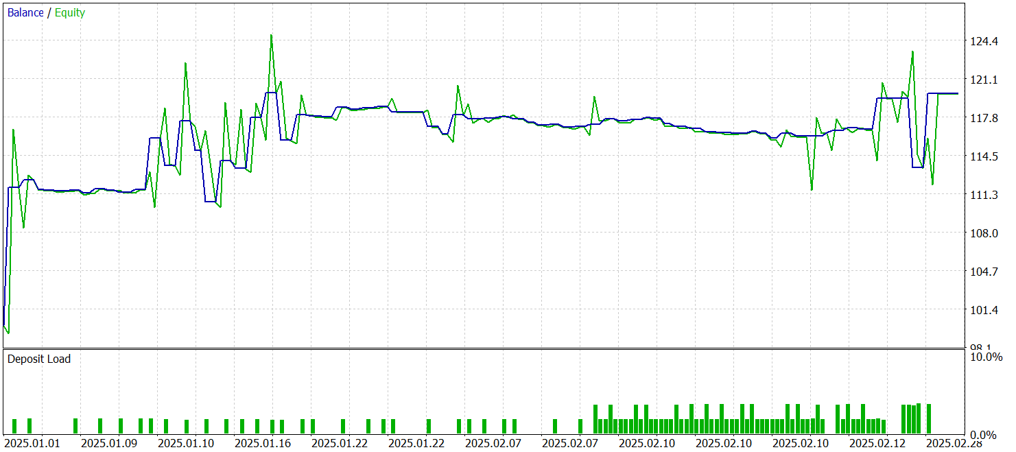
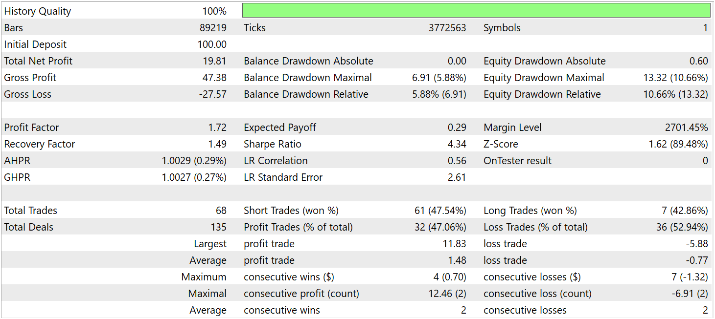
During the testing period, the model executed 68 trades, of which 32 were closed in profit, corresponding to a win rate of slightly above 47%. At the same time, the average profit per winning trade was nearly twice as large as the average loss per losing trade. As a result, the model achieved overall profitability over the test period, with a profit factor of 1.72.
Conclusion
Across these two articles, we explored the theoretical foundations of the CATCH framework, an innovative approach that combines Fourier transform techniques with frequency-domain patching mechanisms for anomaly detection in multivariate time series. Its main advantage lies in its ability to uncover complex patterns that remain hidden when analysis is performed solely in the time domain.
Representing data in the frequency domain provides deeper insight into market dynamics. The frequency patching mechanism introduces flexibility into the analysis, enabling the model to adapt to changing conditions in the observed environment. Unlike classical methods, CATCH is not limited to detecting sharp price spikes or outliers, but is capable of identifying latent dependencies within the data.
In the practical section, we implemented our own version of the proposed approach in MQL5, trained the model, and tested it on real historical data. The results indicate promising potential; however, several questions regarding further optimization remain open.
References
- CATCH: Channel-Aware multivariate Time Series Anomaly Detection via Frequency Patching
- Other articles from this series
Programs Used in the Article
| # | Name | Type | Description |
|---|---|---|---|
| 1 | Research.mq5 | Expert Advisor | Expert Advisor for collecting samples |
| 2 | ResearchRealORL.mq5 | Expert Advisor | Expert Advisor for collecting samples using the Real-ORL method |
| 3 | Study.mq5 | Expert Advisor | Model training Expert Advisor |
| 4 | Test.mq5 | Expert Advisor | Model Testing Expert Advisor |
| 5 | Trajectory.mqh | Class library | System state and model architecture description structure |
| 6 | NeuroNet.mqh | Class library | A library of classes for creating a neural network |
| 7 | NeuroNet.cl | Code library | OpenCL program code |
Translated from Russian by MetaQuotes Ltd.
Original article: https://www.mql5.com/ru/articles/17675
Warning: All rights to these materials are reserved by MetaQuotes Ltd. Copying or reprinting of these materials in whole or in part is prohibited.
This article was written by a user of the site and reflects their personal views. MetaQuotes Ltd is not responsible for the accuracy of the information presented, nor for any consequences resulting from the use of the solutions, strategies or recommendations described.

- Free trading apps
- Over 8,000 signals for copying
- Economic news for exploring financial markets
You agree to website policy and terms of use