
Neural Networks in Trading: Generalized 3D Referring Expression Segmentation

Introduction
3D Referring Expression Segmentation (3D-RES) is an emerging area within the multimodal field that has garnered significant interest from researchers. This task focuses on segmenting target instances based on given natural language expressions. However, traditional 3D-RES approaches are limited to scenarios involving a single target, significantly constraining their practical applicability. In real-world settings, instructions often result in situations where the target cannot be found or where multiple targets need to be identified simultaneously. This reality presents a problem that existing 3D-RES models cannot handle. To address this gap, the authors of "3D-GRES: Generalized 3D Referring Expression Segmentation" have proposed a novel method called Generalized 3D Referring Expression Segmentation (3D-GRES), designed to interpret instructions that reference an arbitrary number of targets.
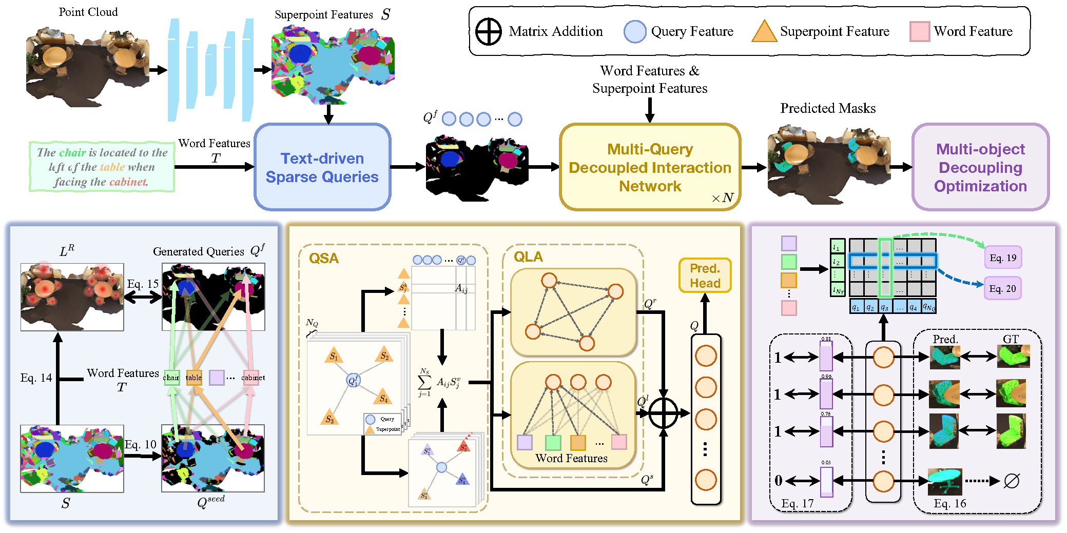
The primary objective of 3D-GRES is to accurately identify multiple targets within a group of similar objects. The key to solving such tasks is to decompose the problem in a way that enables multiple queries to simultaneously process the localization of multi-object language instructions. Each query is responsible for a single instance in a multi-object scene. The authors of 3D-GRES introduced the Multi-Query Decoupled Interaction Network (MDIN), a module designed to streamline interaction among queries, superpoints, and text. To effectively manage an arbitrary number of targets, a mechanism was introduced that enables multiple queries to operate independently while jointly generating multi-object outputs. Each query here is responsible for a single target within the multi-instance context.
To uniformly cover key targets in the point cloud by the learnable queries, the authors proposed a new Text-Guided Sparse Query (TSQ) module, which utilizes textual referring expressions. Additionally, to simultaneously achieve distinctiveness among queries and maintain overall semantic consistency, the authors developed an optimization strategy called Multi-Object Decoupling Optimization (MDO). This strategy decomposes a multi-object mask into individual single-object supervisions, preserving the discriminative power of each query. The alignment between query functions and the superpoint features in the point cloud with textual semantics ensures semantic consistency across multiple targets.
1. The 3D-GRES Algorithm
The classical 3D-RES task is focused on generating a 3D mask for a single target object within a point cloud scene, guided by a referring expression. This traditional formulation has significant limitations. First, it is not suitable for scenarios in which no object in the point cloud matches the given expression. Second, it does not account for cases where multiple objects meet the described criteria. This substantial gap between model capabilities and real-world applicability restricts the practical use of 3D-RES technologies.
To overcome these limitations, the Generalized 3D Referring Expression Segmentation (3D-GRES) method was proposed, designed to identify an arbitrary number of objects from textual descriptions. 3D-GRES analyzes a 3D point cloud scene P and a referring expression E. This produces corresponding 3D masks M, which may be empty or contain one or more objects. This method enables the identification of multiple objects using multi-target expressions and supports "nothing" expressions to verify the absence of target objects, thereby offering enhanced flexibility and robustness in object retrieval and interaction.
3D-GRES first processes the input referring expression by encoding it into text tokens 𝒯 using a pre-trained RoBERTa model. To facilitate multimodal alignment, the encoded tokens are projected into a multimodal space of dimension D. Positional encoding is applied to the resulting representations.
For the input point cloud with positions P and features F, superpoints are extracted using a sparse 3D U-Net and are projected into the same D-dimensional multimodal space.
Multi-Query Decoupled Interaction Network (MDIN) utilizes multiple queries to handle individual instances within multi-object scenes, aggregating them into a final result. In scenes without target objects, predictions rely on the confidence scores of each query—if all queries have low confidence, a null output is predicted.
MDIN consists of several identical modules, each comprising a Query-Superpoint Aggregation (QSA) module and a Query-Language Aggregation (QLA) module, which facilitate interaction among Query, Superpoints, and the text. Unlike previous models that use random Query initialization, MDIN uses a Text-Guided Sparse Query (TSQ) module, to generate text-driven sparse Query, ensuring efficient scene coverage. Additionally, the Multi-Object Decoupling Optimization (MDO) strategy supports multiple queries.
Query can be vied as an anchor within the point cloud space. Through interaction with Superpoints, Queries capture the global context of the point cloud. Notably, selected Superpoints act as queries during the interaction process, enhancing local aggregation. This localized focus supports effective decoupling of queries.
Initially, a similarity distribution is computed between the Superpoint features S and query embeddings Qf. Queries then aggregate relevant Superpoints based on these similarity scores. The updated scene representation, now informed by Qs is passed to the QLA module to model Query-Query and Query-Language interactions. QLA includes a Self-Attention block for query features Qs and a multimodal cross-attention block to capture dependencies between each word and each query.
The query features with relation context Qr, language-aware features Ql and scene-informed features Qs are then summed and fused using an MLP.
To ensure a sparse distribution of initialized queries across the point cloud scene while preserving essential geometric and semantic information, the authors of 3D-GRES apply Furthest Point Sampling directly on the Superpoints.
To further enhance query separation and assignment to distinct objects, the method leverages intrinsic attributes of queries generated by TSQ. Each query originates from a specific Superpoint in the point cloud, inherently linking it to a corresponding object. Queries associated with target instances handle segmentation for those instances, while unrelated objects are assigned to the nearest query. This approach uses preliminary visual constraints to disentangle queries and assign them to distinct targets.
A visual representation of the 3D-GRES method, as presented by the authors, is shown below.
2. Implementation in MQL5
After considering the theoretical aspects of the 3D-GRES method, we move on to the practical part of our article, in which we implement our vision of the proposed approaches using MQL5. First, let us consider what distinguishes the 3D-GRES algorithm from the methods we previously examined, and what they have in common.
First of all, it is the multimodality of the 3D-GRES method. This is the first time we encounter referring expressions that aim to make the analysis more targeted. And we will certainly take advantage of this idea. However, instead of using a language model, we will encode account state and open positions as input to the model. Thus, depending on the embedding of the account state, the model will be guided to search for entry or exit points.
Another important point worth highlighting is the way trainable queries are handled. Like the models we previously reviewed, 3D-GRES uses a set of trainable queries. There is a difference in the principle of their formation. SPFormer and MAFT use static queries optimized during training and fixed during inference. Thus, the model learned some patterns and then acted according to a "prepared scheme". The authors of 3D-GRES propose generating queries based on the input data, making them more localized and dynamic. To ensure optimal coverage of the analyzed scene space, various heuristics are applied. We will also apply this idea in our implementation.
Furthermore, positional encoding of tokens is used in 3D-GRES. This is similar to the MAFT method and serves as a basis for our choice of parent class in the implementation. With that foundation, we begin by extending our OpenCL program.
2.1 Query Diversification
To ensure maximum spatial coverage of the scene by trainable queries, we introduce a diversity loss, designed to "repel" queries from their neighbors:
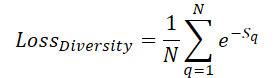
Here Sq denotes the distance to query q. Clearly, when S=0, the loss equals 1. As the average distance between queries increases, the loss tends toward 0. Consequently, during training, the model will spread queries more uniformly.
However, our focus is not on the value of the loss itself, but rather on the direction of the gradient, which adjusts the query parameters to maximize their separation from one another. In our implementation, we immediately compute the error gradient and add it to the main backpropagation flow, allowing to optimize the parameters accordingly. This algorithm is implemented in the DiversityLoss kernel.
This kernel takes two global data buffers and two scalar variables as parameters. The first buffer contains the current query features, and the second buffer will store the computed gradients of the diversity loss.
__kernel void DiversityLoss(__global const float *data,
                            __global float *grad,
                            const int activation,
                            const int add
                           )
  {
   const size_t main = get_global_id(0);
   const size_t slave = get_local_id(1);
   const size_t dim = get_local_id(2);
   const size_t total = get_local_size(1);
   const size_t dimension = get_local_size(2);
Our kernel will operate within a three-dimensional work-space. The first two dimensions correspond to the number of queries being analyzed, while the third dimension represents the size of the feature vector for each query. To minimize access to slower global memory, we will group threads into work-groups along the last two dimensions of the task space.
Inside the kernel body, as usual, we begin by identifying the current thread across all three dimensions of the global task space. Next, we declare a local memory array to facilitate data sharing among threads within a work-group.
__local float Temp[LOCAL_ARRAY_SIZE];
We also determine the offset in the global data buffers to the analyzed values.
   const int shift_main = main * dimension + dim;
   const int shift_slave = slave * dimension + dim;
After that, we load the values from the global data buffers and determine the deviation between them.
   const int value_main = data[shift_main];
   const int value_slave = data[shift_slave];
   float delt = value_main - value_slave;
Note that the task space and work groups are organized such that each thread reads only 2 values from global memory. Next, we need to collect the sum of the distances from all the flows. To do this, we first organize a loop to collect the sum of individual values in the elements of the local array.
   for(int d = 0; d < dimension; d++)
     {
      for(int i = 0; i < total; i += LOCAL_ARRAY_SIZE)
        {
         if(d == dim)
           {
            if(i <= slave && (i + LOCAL_ARRAY_SIZE) > slave)
              {
               int k = i % LOCAL_ARRAY_SIZE;
               float val = pow(delt, 2.0f) / total;
               if(isinf(val) || isnan(val))
                  val = 0;
               Temp[k] = ((d == 0 && i == 0) ? 0 : Temp[k]) + val;
              }
           }
         barrier(CLK_LOCAL_MEM_FENCE);
        }
     }
It is worth noting that we initially store the simple difference between two values in a variable called delt. Only just before adding the distance to the local array do we square this value. This design choice is intentional: the derivative of our loss function involves the raw difference itself. So we preserve it in its original form to avoid redundant recalculation later.
In the next step, we accumulate the sum of all values in our local array.
   const int ls = min((int)total, (int)LOCAL_ARRAY_SIZE);
   int count = ls;
   do
     {
      count = (count + 1) / 2;
      if(slave < count)
        {
         Temp[slave] += ((slave + count) < ls ? Temp[slave + count] : 0);
         if(slave + count < ls)
            Temp[slave + count] = 0;
        }
      barrier(CLK_LOCAL_MEM_FENCE);
     }
   while(count > 1);
Only then do we calculate the value of the diversification error of the analyzed query and the error gradient of the corresponding element.
   float loss = exp(-Temp[0]);
   float gr = 2 * pow(loss, 2.0f) * delt / total;
   if(isnan(gr) || isinf(gr))
      gr = 0;
After that, we have an exciting path ahead of us: collecting error gradients in terms of individual features of the analyzed query. The algorithm for summing error gradients is similar to that described above for summing distances.
   for(int d = 0; d < dimension; d++)
     {
      for(int i = 0; i < total; i += LOCAL_ARRAY_SIZE)
        {
         if(d == dim)
           {
            if(i <= slave && (i + LOCAL_ARRAY_SIZE) > slave)
              {
               int k = i % LOCAL_ARRAY_SIZE;
               Temp[k] = ((d == 0 && i == 0) ? 0 : Temp[k]) + gr;
              }
           }
         barrier(CLK_LOCAL_MEM_FENCE);
        }
      //---
      int count = ls;
      do
        {
         count = (count + 1) / 2;
         if(slave < count && d == dim)
           {
            Temp[slave] += ((slave + count) < ls ? Temp[slave + count] : 0);
            if(slave + count < ls)
               Temp[slave + count] = 0;
           }
         barrier(CLK_LOCAL_MEM_FENCE);
        }
      while(count > 1);
      if(slave == 0 && d == dim)
        {
         if(isnan(Temp[0]) || isinf(Temp[0]))
            Temp[0] = 0;
         if(add > 0)
            grad[shift_main] += Deactivation(Temp[0],value_main,activation);
         else
            grad[shift_main] = Deactivation(Temp[0],value_main,activation);
        }
      barrier(CLK_LOCAL_MEM_FENCE);
     }
  }
It is important to note that the algorithm described above combines both the feed-forward and backpropagation pass iterations. This integration allows us to use the algorithm exclusively during model training, eliminating these operations during inference. As a result, this optimization has a positive impact on decision-making time in production scenarios.
With this, we complete our work on the OpenCL program and move on to constructing the class that will implement the core ideas of the 3D-GRES method.
2.2 The 3D-GRES Method Class
To implement the approaches proposed in the 3D-GRES method, we will create a new object in the main program: CNeuronGRES. As previously mentioned, its core functionality will be inherited from the CNeuronMAFT class. The structure of the new class is shown below.
class CNeuronGRES :  public CNeuronMAFT
  {
protected:
   CLayer            cReference;
   CLayer            cRefKey;
   CLayer            cRefValue;
   CLayer            cMHRefAttentionOut;
   CLayer            cRefAttentionOut;
   //---
   virtual bool      CreateBuffers(void);
   virtual bool      DiversityLoss(CNeuronBaseOCL *neuron, const int units,
                                   const int dimension, const bool add = false);
   //---
   virtual bool      feedForward(CNeuronBaseOCL *NeuronOCL) override { return false; }
   virtual bool      feedForward(CNeuronBaseOCL *NeuronOCL, CBufferFloat *SecondInput) override;
   //---
   virtual bool      calcInputGradients(CNeuronBaseOCL *NeuronOCL) override { return false; }
   virtual bool      calcInputGradients(CNeuronBaseOCL *NeuronOCL, CBufferFloat *SecondInput,
                                        CBufferFloat *SecondGradient, ENUM_ACTIVATION SecondActivation = None)
                                        override;
   virtual bool      updateInputWeights(CNeuronBaseOCL *NeuronOCL) override { return false; }
   virtual bool      updateInputWeights(CNeuronBaseOCL *NeuronOCL, CBufferFloat *SecondInput) override;

public:
                     CNeuronGRES(void) {};
                    ~CNeuronGRES(void) {};
   //---
   virtual bool      Init(uint numOutputs, uint myIndex, COpenCLMy *open_cl,
                          uint window, uint window_key, uint units_count, uint heads,
                          uint window_sp, uint units_sp, uint heads_sp,
                          uint ref_size, uint layers, uint layers_to_sp,
                          ENUM_OPTIMIZATION optimization_type, uint batch);
   //---
   virtual int       Type(void) override   const   {  return defNeuronGRES; }
   //---
   virtual bool      Save(int const file_handle) override;
   virtual bool      Load(int const file_handle) override;
   //---
   virtual bool      WeightsUpdate(CNeuronBaseOCL *source, float tau) override;
   virtual void      SetOpenCL(COpenCLMy *obj) override;
  };
Alongside the core functionality, we also inherit a broad range of internal objects from the parent class, which will cover most of our requirements. Most, but not all. To address the remaining needs, we introduce additional objects for handling referring expressions. All objects in this class are declared as static, allowing us to keep both the constructor and destructor empty. Initialization of all declared and inherited components is handled within the Init method, which receives the key constants required to unambiguously define the architecture of the constructed object.
bool CNeuronGRES::Init(uint numOutputs, uint myIndex, COpenCLMy *open_cl,
                       uint window, uint window_key, uint units_count, uint heads,
                       uint window_sp, uint units_sp, uint heads_sp,
                       uint ref_size, uint layers, uint layers_to_sp,
                       ENUM_OPTIMIZATION optimization_type, uint batch
                      )
  {
   if(!CNeuronBaseOCL::Init(numOutputs, myIndex, open_cl, window * units_count, optimization_type, batch))
      return false;
Unfortunately, the structure of our new class differs significantly from the parent class, which prevents full reuse of all inherited methods. This is also reflected in the logic of the initialization method. Here we must initialize not only the added components but also the inherited ones manually.
In the Init method body, we begin by calling the base class's identically named initialization method, which performs the initial validation of input parameters and activates data exchange interfaces between neural layers for model operation.
After that, we store the received parameters in the internal variables of our class.
   iWindow = window;
   iUnits = units_count;
   iHeads = heads;
   iSPUnits = units_sp;
   iSPWindow = window_sp;
   iSPHeads = heads_sp;
   iWindowKey = window_key;
   iLayers = MathMax(layers, 1);
   iLayersSP = MathMax(layers_to_sp, 1);
Here we will also declare several variables for temporary storage of pointers to objects of various neural layers, which we will initialize within our method.
   CNeuronBaseOCL *base = NULL;
   CNeuronTransposeOCL *transp = NULL;
   CNeuronConvOCL *conv = NULL;
   CNeuronLearnabledPE *pe = NULL;
Next, we move on to constructing the trainable query generation modules. It's worth recalling that the authors of 3D-GRES proposed generating dynamic queries based on the input point cloud. However, the analyzed point cloud may differ from the set of trainable queries both in the number of elements and in the dimensionality of feature vectors per element. We address this challenge in two stages. First, we transpose the original data tensor and use a convolutional layer to change the number of elements in the sequence. Using a convolutional layer allows us to perform this operation within independent univariate sequences.
//--- Init Querys
   cQuery.Clear();
   transp = new CNeuronTransposeOCL();
   if(!transp ||
      !transp.Init(0, 0, OpenCL, iSPUnits, iSPWindow, optimization, iBatch) ||
      !cQuery.Add(transp))
      return false;
   conv = new CNeuronConvOCL();
   if(!conv ||
      !conv.Init(0, 1, OpenCL, iSPUnits, iSPUnits, iUnits, 1, iSPWindow, optimization, iBatch) ||
      !cQuery.Add(conv))
      return false;
   conv.SetActivationFunction(SIGMOID);
In the second stage, we perform the inverse transposition of the tensor and make its projection into the multimodal space.
   transp = new CNeuronTransposeOCL();
   if(!transp ||
      !transp.Init(0, 2, OpenCL, iSPWindow, iUnits, optimization, iBatch) ||
      !cQuery.Add(transp))
      return false;
   conv = new CNeuronConvOCL();
   if(!conv ||
      !conv.Init(0, 3, OpenCL, iSPWindow, iSPWindow, iWindow, iUnits, 1, optimization, iBatch) ||
      !cQuery.Add(conv))
      return false;
   conv.SetActivationFunction(SIGMOID);
Now we just need to add fully trainable positional encoding.
   pe = new CNeuronLearnabledPE();
   if(!pe ||
      !pe.Init(0, 4, OpenCL, iWindow * iUnits, optimization, iBatch) ||
      !cQuery.Add(pe))
      return false;
Similar to the algorithm of the parent class, we will place the positional encoding data of requests in a separate information flow.
   base = new CNeuronBaseOCL();
   if(!base ||
      !base.Init(0, 5, OpenCL, pe.Neurons(), optimization, iBatch) ||
      !base.SetOutput(pe.GetPE()) ||
      !cQPosition.Add(base))
      return false;
The algorithm for generating the Superpoints model architecture has been completely copied it from the parent class without any changes.
//--- Init SuperPoints
   int layer_id = 6;
   cSuperPoints.Clear();
   for(int r = 0; r < 4; r++)
     {
      if(iSPUnits % 2 == 0)
        {
         iSPUnits /= 2;
         CResidualConv *residual = new CResidualConv();
         if(!residual ||
            !residual.Init(0, layer_id, OpenCL, 2 * iSPWindow, iSPWindow, iSPUnits, optimization, iBatch) ||
            !cSuperPoints.Add(residual))
            return false;
        }
      else
        {
         iSPUnits--;
         conv = new CNeuronConvOCL();
         if(!conv ||
            !conv.Init(0, layer_id, OpenCL, 2 * iSPWindow, iSPWindow, iSPWindow, iSPUnits, 1, optimization,
                                                                                                 iBatch) ||
            !cSuperPoints.Add(conv))
            return false;
         conv.SetActivationFunction(SIGMOID);
        }
      layer_id++;
     }
   conv = new CNeuronConvOCL();
   if(!conv ||
      !conv.Init(0, layer_id, OpenCL, iSPWindow, iSPWindow, iWindow, iSPUnits, 1, optimization, iBatch) ||
      !cSuperPoints.Add(conv))
      return false;
   conv.SetActivationFunction(SIGMOID);
   layer_id++;
   pe = new CNeuronLearnabledPE();
   if(!pe ||
      !pe.Init(0, layer_id, OpenCL, conv.Neurons(), optimization, iBatch) ||
      !cSuperPoints.Add(pe))
      return false;
   layer_id++;
And to generate the embedding of the referring expression, we use a fully connected MLP with an added positional encoding layer.
//--- Reference
   cReference.Clear();
   base = new CNeuronBaseOCL();
   if(!base ||
      !base.Init(iWindow * iUnits, layer_id, OpenCL, ref_size, optimization, iBatch) ||
      !cReference.Add(base))
      return false;
   layer_id++;
   base = new CNeuronBaseOCL();
   if(!base ||
      !base.Init(0, layer_id, OpenCL, iWindow * iUnits, optimization, iBatch) ||
      !cReference.Add(base))
      return false;
   base.SetActivationFunction(SIGMOID);
   layer_id++;
   pe = new CNeuronLearnabledPE();
   if(!pe ||
      !pe.Init(0, layer_id, OpenCL, base.Neurons(), optimization, iBatch) ||
      !cReference.Add(pe))
      return false;
   layer_id++;
It is important to note that the output of the MLP produces a tensor dimensionally aligned with the trainable query tensor. This design allows us to decompose the referring expression into multiple semantic components, enabling a more comprehensive analysis of the current market situation.
At this point, we have completed the initialization of objects responsible for the primary processing of input data. Next, we proceed to the initialization loop for the internal neural layer objects. Before that, however, we clear the internal object collection arrays to ensure a clean setup.
//--- Inside layers
   cQKey.Clear();
   cQValue.Clear();
   cSPKey.Clear();
   cSPValue.Clear();
   cSelfAttentionOut.Clear();
   cCrossAttentionOut.Clear();
   cMHCrossAttentionOut.Clear();
   cMHSelfAttentionOut.Clear();
   cMHRefAttentionOut.Clear();
   cRefAttentionOut.Clear();
   cRefKey.Clear();
   cRefValue.Clear();
   cResidual.Clear();
   for(uint l = 0; l < iLayers; l++)
     {
      //--- Cross-Attention
      //--- Query
      conv = new CNeuronConvOCL();
      if(!conv ||
         !conv.Init(0,layer_id, OpenCL, iWindow, iWindow, iWindowKey*iHeads, iUnits, 1,optimization, iBatch) ||
         !cQuery.Add(conv))
         return false;
      layer_id++;
In the loop body, we first initialize the cross-attention Query Superpoint objects. Here we create a Query entity generation object for the attention block. And then, if necessary, we add objects for generating Key and Value entities.
      if(l % iLayersSP == 0)
        {
         //--- Key
         conv = new CNeuronConvOCL();
         if(!conv ||
            !conv.Init(0, layer_id, OpenCL, iWindow, iWindow, iWindowKey * iSPHeads, iSPUnits, 1,
                                                                             optimization, iBatch) ||
            !cSPKey.Add(conv))
            return false;
         layer_id++;
         //--- Value
         conv = new CNeuronConvOCL();
         if(!conv ||
            !conv.Init(0, layer_id, OpenCL, iWindow, iWindow, iWindowKey * iSPHeads, iSPUnits, 1,
                                                                             optimization, iBatch) ||
            !cSPValue.Add(conv))
            return false;
         layer_id++;
        }
We add a layer for recording the results of multi-headed attention.
      //--- Multy-Heads Attention Out
      base = new CNeuronBaseOCL();
      if(!base ||
         !base.Init(0, layer_id, OpenCL, iWindowKey * iHeads * iUnits, optimization, iBatch) ||
         !cMHCrossAttentionOut.Add(base))
         return false;
      layer_id++;
And a result scaling layer.
      //--- Cross-Attention Out
      conv = new CNeuronConvOCL();
      if(!conv ||
         !conv.Init(0, layer_id, OpenCL, iWindowKey * iHeads, iWindowKey * iHeads, iWindow, iUnits, 1,
                                                                                 optimization, iBatch) ||
         !cCrossAttentionOut.Add(conv))
         return false;
      layer_id++;
The cross-attention block ends with a layer of residual connections.
      //--- Residual
      base = new CNeuronBaseOCL();
      if(!base ||
         !base.Init(0, layer_id, OpenCL, iWindow * iUnits, optimization, iBatch) ||
         !cResidual.Add(base))
         return false;
      layer_id++;
In the next step, we initialize the Self-Attention block to analyze Query-Query dependencies. Here we generate all entities based on the results of the previous cross-attention block.
      //--- Self-Attention
      //--- Query
      conv = new CNeuronConvOCL();
      if(!conv ||
         !conv.Init(0,layer_id, OpenCL, iWindow, iWindow, iWindowKey*iHeads, iUnits, 1, optimization, iBatch) ||
         !cQuery.Add(conv))
         return false;
      layer_id++;
      //--- Key
      conv = new CNeuronConvOCL();
      if(!conv ||
         !conv.Init(0,layer_id, OpenCL, iWindow, iWindow, iWindowKey*iHeads, iUnits, 1, optimization, iBatch) ||
         !cQKey.Add(conv))
         return false;
      layer_id++;
      //--- Value
      conv = new CNeuronConvOCL();
      if(!conv ||
         !conv.Init(0,layer_id, OpenCL, iWindow, iWindow, iWindowKey*iHeads, iUnits, 1, optimization, iBatch) ||
         !cQValue.Add(conv))
         return false;
      layer_id++;
In this case, for each internal layer we generate all entities with the same number of attention heads.
Add a layer for recording the results of multi-headed attention.
      //--- Multy-Heads Attention Out
      base = new CNeuronBaseOCL();
      if(!base ||
         !base.Init(0, layer_id, OpenCL, iWindowKey * iHeads * iUnits, optimization, iBatch) ||
         !cMHSelfAttentionOut.Add(base))
         return false;
      layer_id++;
And a result scaling layer.
      //--- Self-Attention Out
      conv = new CNeuronConvOCL();
      if(!conv ||
         !conv.Init(0, layer_id, OpenCL, iWindowKey * iHeads, iWindowKey * iHeads, iWindow, iUnits, 1,
                                                                                  optimization, iBatch) ||
         !cSelfAttentionOut.Add(conv))
         return false;
      layer_id++;
In parallel with the Self-Attention block there is the Query cross-attention block to semantic referring expressions. The Query entity here is generated based on the results of the previous cross-attention block.
      //--- Reference Cross-Attention
      //--- Query
      conv = new CNeuronConvOCL();
      if(!conv ||
         !conv.Init(0,layer_id, OpenCL, iWindow, iWindow, iWindowKey*iHeads, iUnits, 1, optimization, iBatch) ||
         !cQuery.Add(conv))
         return false;
      layer_id++;
The Key-Value tensor is formed from previously prepared semantic embeddings.
      //--- Key
      conv = new CNeuronConvOCL();
      if(!conv ||
         !conv.Init(0,layer_id, OpenCL, iWindow, iWindow, iWindowKey*iHeads, iUnits, 1, optimization, iBatch) ||
         !cRefKey.Add(conv))
         return false;
      layer_id++;
      //--- Value
      conv = new CNeuronConvOCL();
      if(!conv ||
         !conv.Init(0,layer_id, OpenCL, iWindow, iWindow, iWindowKey*iHeads, iUnits, 1, optimization, iBatch) ||
         !cRefValue.Add(conv))
         return false;
      layer_id++;
Similar to the Self-Attention block, we generate all entities on each new layer with an equal number of attention heads.
Next, we add layers of multi-headed attention results and result scaling.
      //--- Multy-Heads Attention Out
      base = new CNeuronBaseOCL();
      if(!base ||
         !base.Init(0, layer_id, OpenCL, iWindowKey * iHeads * iUnits, optimization, iBatch) ||
         !cMHRefAttentionOut.Add(base))
         return false;
      layer_id++;
      //--- Cross-Attention Out
      conv = new CNeuronConvOCL();
      if(!conv ||
         !conv.Init(0,layer_id, OpenCL, iWindowKey*iHeads, iWindowKey*iHeads, iWindow, iUnits, 1,
                                                                             optimization, iBatch) ||
         !cRefAttentionOut.Add(conv))
         return false;
      layer_id++;
      if(!conv.SetGradient(((CNeuronBaseOCL*)cSelfAttentionOut[cSelfAttentionOut.Total() - 1]).getGradient(),
                                                                                                        true))
         return false;
This block is completed by a layer of residual connections, which combines the results of all three attention blocks.
      //--- Residual
      base = new CNeuronBaseOCL();
      if(!base || !base.Init(0, layer_id, OpenCL, iWindow * iUnits, optimization, iBatch))
         return false;
      if(!cResidual.Add(base))
         return false;
      layer_id++;
The final processing of enriched queries is implemented in the FeedForward block with residual connections. Its structure is similar to the vanilla Transformer.
      //--- Feed Forward
      conv = new CNeuronConvOCL();
      if(!conv ||
         !conv.Init(0, layer_id, OpenCL, iWindow, iWindow, 4*iWindow, iUnits, 1, optimization, iBatch))
         return false;
      conv.SetActivationFunction(LReLU);
      if(!cFeedForward.Add(conv))
         return false;
      layer_id++;
      conv = new CNeuronConvOCL();
      if(!conv ||
         !conv.Init(0, layer_id, OpenCL, 4 * iWindow, 4 * iWindow, iWindow, iUnits, 1, optimization, iBatch))
         return false;
      if(!cFeedForward.Add(conv))
         return false;
      layer_id++;
      //--- Residual
      base = new CNeuronBaseOCL();
      if(!base || !base.Init(0, layer_id, OpenCL, iWindow * iUnits, optimization, iBatch))
         return false;
      if(!base.SetGradient(conv.getGradient()))
         return false;
      if(!cResidual.Add(base))
         return false;
      layer_id++;
In addition, we will transfer from the parent class the algorithm for correcting the object centers. Note that this object was provided by the authors of the 3D-GRES method.
      //--- Delta position
      conv = new CNeuronConvOCL();
      if(!conv || !conv.Init(0, layer_id, OpenCL, iWindow, iWindow, iWindow, iUnits, 1, optimization, iBatch))
         return false;
      conv.SetActivationFunction(SIGMOID);
      if(!cQPosition.Add(conv))
         return false;
      layer_id++;
      base = new CNeuronBaseOCL();
      if(!base || !base.Init(0, layer_id, OpenCL, conv.Neurons(), optimization, iBatch))
         return false;
      if(!base.SetGradient(conv.getGradient()))
         return false;
      if(!cQPosition.Add(base))
         return false;
      layer_id++;
     }
We now move on to the next iteration of the loop creating objects of the inner layer. After all loop iterations have been successfully completed, we replace the pointers to the data buffers, which allows us to reduce the number of data copying operations and speed up the learning process.
   base = cResidual[iLayers * 3 - 1];
   if(!SetGradient(base.getGradient()))
      return false;
//---
   SetOpenCL(OpenCL);
//---
   return true;
  }
At the end of the method operations, we return a boolean result to the calling program, indicating the success or failure of the executed steps.
It is worth noting that, just like in our previous article, we have moved the creation of auxiliary data buffers into a separate method called CreateBuffers. I encourage you to review this method independently. Its full source code is available in the attachment.
Once the object of our new class has been initialized, we proceed to construct the feed-forward pass algorithm, which is implemented in the feedForward method. This time, the method accepts two pointers to input data objects. One of them contains the analyzed point cloud, and the other representing the referring expression.
bool CNeuronGRES::feedForward(CNeuronBaseOCL *NeuronOCL, CBufferFloat *SecondInput)
  {
//--- Superpoints
   CNeuronBaseOCL *superpoints = NeuronOCL;
   int total_sp = cSuperPoints.Total();
   for(int i = 0; i < total_sp; i++)
     {
      if(!cSuperPoints[i] ||
         !((CNeuronBaseOCL*)cSuperPoints[i]).FeedForward(superpoints))
         return false;
      superpoints = cSuperPoints[i];
     }
In the body of the method, we immediately organize a feed-forward loop of our small Superpoints generation model. Similarly, we generate queries.
//--- Query
   CNeuronBaseOCL *query = NeuronOCL;
   for(int i = 0; i < 5; i++)
     {
      if(!cQuery[i] ||
         !((CNeuronBaseOCL*)cQuery[i]).FeedForward(query))
         return false;
      query = cQuery[i];
     }
Generating the tensor of semantic embeddings for the referring expression requires a bit more work. The referring expression is received as a raw data buffer. But the internal modules in the feed-forward pass expect a neural layer object as input. Therefore, we use the first layer of the internal semantic embedding generator model as a placeholder to receive the input data, similar to how we handle inputs in the main model. However, in this case, we do not copy the buffer contents entirely; instead, we substitute the underlying data pointers with those from the buffer.
//--- Reference
   CNeuronBaseOCL *reference = cReference[0];
   if(!SecondInput)
      return false;
   if(reference.getOutput() != SecondInput)
      if(!reference.SetOutput(SecondInput, true))
         return false;
Next, we run a feed-forward loop for the internal model.
   for(int i = 1; i < cReference.Total(); i++)
     {
      if(!cReference[i] ||
         !((CNeuronBaseOCL*)cReference[i]).FeedForward(reference))
         return false;
      reference = cReference[i];
     }
This completes the preliminary processing of the source data and we can move on to the main data decoding algorithm. For this, we organize a loop through the internal layers of the Decoder.
   CNeuronBaseOCL *inputs = query, *key = NULL, *value = NULL, *base = NULL, *cross = NULL, *self = NULL;
//--- Inside layers
   for(uint l = 0; l < iLayers; l++)
     {
      //--- Calc Position bias
      cross = cQPosition[l * 2];
      if(!cross ||
         !CalcPositionBias(cross.getOutput(),
                           ((CNeuronLearnabledPE*)superpoints).GetPE(), cPositionBias[l],
                           iUnits, iSPUnits, iWindow))
         return false;
We begin by defining the positional offset coefficients, following the approach used in the MAFT method. This represents a departure from the original 3D-GRES algorithm, in which the authors used an MLP to generate the attention mask.
Next, we proceed to the cross-attention block QSA, which is responsible for modeling Query–Superpoint dependencies. In this block, we first generate the tensors for the Query, Key, and Value entities. The latter two are generated only when necessary.
      //--- Cross-Attention
      query = cQuery[l * 3 + 5];
      if(!query || !query.FeedForward(inputs))
         return false;
      key = cSPKey[l / iLayersSP];
      value = cSPValue[l / iLayersSP];
      if(l % iLayersSP == 0)
        {
         if(!key || !key.FeedForward(superpoints))
            return false;
         if(!value || !value.FeedForward(cSuperPoints[total_sp - 2]))
            return false;
        }
Then we analyze dependencies taking into account the positional bias coefficients.
      if(!AttentionOut(query, key, value, cScores[l * 3], cMHCrossAttentionOut[l], cPositionBias[l],
                                               iUnits, iHeads, iSPUnits, iSPHeads, iWindowKey, true))
         return false;
We scale the results of multi-headed attention and add residual connection values, followed by data normalization.
      base = cCrossAttentionOut[l];
      if(!base || !base.FeedForward(cMHCrossAttentionOut[l]))
         return false;
      value = cResidual[l * 3];
      if(!value ||
         !SumAndNormilize(inputs.getOutput(), base.getOutput(), value.getOutput(), iWindow, false, 0, 0, 0, 1)||
         !SumAndNormilize(cross.getOutput(), value.getOutput(), value.getOutput(), iWindow, true, 0, 0, 0, 1))
         return false;
      inputs = value;
In the next step, we organize operations of the QLA module. Here we need to organize a feed-forward pass two attention blocks:
- Self-Attention → Query-Query;
- Cross-Attention → Query-Reference.
First, we implement the operations of the Self-Attention block. Here we generate Query, Key and Value entity tensors in full, based on the data received from the previous Decoder block.
      //--- Self-Atention
      query = cQuery[l * 3 + 6];
      if(!query || !query.FeedForward(inputs))
         return false;
      key = cQKey[l];
      if(!key || !key.FeedForward(inputs))
         return false;
      value = cQValue[l];
      if(!value || !value.FeedForward(inputs))
         return false;
Then we analyze dependencies in the vanilla multi-headed attention module.
      if(!AttentionOut(query, key, value, cScores[l * 3 + 1], cMHSelfAttentionOut[l], -1,
                                        iUnits, iHeads, iUnits, iHeads, iWindowKey, false))
         return false;
      self = cSelfAttentionOut[l];
      if(!self || !self.FeedForward(cMHSelfAttentionOut[l]))
         return false;
After that, we scale the obtained results.
The cross-attention block is constructed in a similar way. The only difference is that Key and Value entities are generated from the semantic embeddings of the referring expression.
      //--- Reference Cross-Attention
      query = cQuery[l * 3 + 7];
      if(!query || !query.FeedForward(inputs))
         return false;
      key = cRefKey[l];
      if(!key || !key.FeedForward(reference))
         return false;
      value = cRefValue[l];
      if(!value || !value.FeedForward(reference))
         return false;
      if(!AttentionOut(query, key, value, cScores[l * 3 + 2], cMHRefAttentionOut[l], -1,
                                       iUnits, iHeads, iUnits, iHeads, iWindowKey, false))
         return false;
      cross = cRefAttentionOut[l];
      if(!cross || !cross.FeedForward(cMHRefAttentionOut[l]))
         return false;
Next, we sum up the results of all three attention blocks and normalize the obtained data.
      value = cResidual[l * 3 + 1];
      if(!value ||
         !SumAndNormilize(cross.getOutput(), self.getOutput(), value.getOutput(), iWindow, false, 0, 0, 0, 1) ||
         !SumAndNormilize(inputs.getOutput(), value.getOutput(), value.getOutput(), iWindow, true, 0, 0, 0, 1))
         return false;
      inputs = value;
This is followed by the FeedForward block of the vanillaTransformer with residual connection and data normalization.
      //--- Feed Forward
      base = cFeedForward[l * 2];
      if(!base || !base.FeedForward(inputs))
         return false;
      base = cFeedForward[l * 2 + 1];
      if(!base || !base.FeedForward(cFeedForward[l * 2]))
         return false;
      value = cResidual[l * 3 + 2];
      if(!value ||
         !SumAndNormilize(inputs.getOutput(), base.getOutput(), value.getOutput(), iWindow, true, 0, 0, 0, 1))
         return false;
      inputs = value;
You might have noticed that the constructed feed-forward pass algorithm is a kind of symbiosis of 3D-GRES and MAFT. So, we just need to add the final touch from the MAFT method – adjustment of query positions.
      //--- Delta Query position
      base = cQPosition[l * 2 + 1];
      if(!base ||
         !base.FeedForward(inputs))
         return false;
      value = cQPosition[(l + 1) * 2];
      query = cQPosition[l * 2];
      if(!value ||
         !SumAndNormilize(query.getOutput(), base.getOutput(), value.getOutput(), iWindow, false, 0, 0, 0,0.5f))
         return false;
     }
After which we move on to the next Decoder layer. After completing iterations through all internal layers of the Decoder, we sum up the enriched query values with their positional encoding. We pass the results to the next layer of our model via basic interfaces.
   value = cQPosition[iLayers * 2];
   if(!value ||
      !SumAndNormilize(inputs.getOutput(), value.getOutput(), Output, iWindow, true, 0, 0, 0, 1))
      return false;
//---
   return true;
  }
At this point, we simply return a boolean result to the calling program, indicating whether the operations were successfully completed.
With that, we conclude the implementation of the feed-forward pass methods and proceed to the backpropagation algorithm. As usual, this process is divided into two stages:
- Gradient distribution (calcInputGradients);
- Optimization of model parameters (updateInputWeights).
In the first stage, we follow the forward pass operations in reverse order to backpropagate the error gradients. In the second stage, we call the corresponding update methods of the internal layers that contain trainable parameters. At first glance, this looks fairly standard. However, there's a particular detail related to query diversification. Therefore, we let's examine the implementation of the calcInputGradients method in greater detail, as it is responsible for distributing the error gradients.
This method receives, as parameters, pointers to three data objects, along with a constant specifying the activation function used for the second input source.
bool CNeuronGRES::calcInputGradients(CNeuronBaseOCL *NeuronOCL, CBufferFloat *SecondInput,
                                     CBufferFloat *SecondGradient, ENUM_ACTIVATION SecondActivation = -1)
  {
   if(!NeuronOCL || !SecondGradient)
      return false;
In the body of the method, we validate only two of the pointers. During the feed-forward pass, we stored the pointer to the second input source. So the absence of a valid pointer in the parameters at this stage is not critical for us. However, this is not the case for the buffer used to store the error gradients. That is why we explicitly check its validity before proceeding.
At this point, we also declare a number of variables to temporarily store pointers to relevant objects. This concludes the preparatory stage of our implementation.
   CNeuronBaseOCL *residual = GetPointer(this), *query = NULL, *key = NULL, *value = NULL,
                   *key_sp = NULL, *value_sp = NULL, *base = NULL;
Next, we organize a reverse loop through the internal layers of the Decoder.
//--- Inside layers
   for(int l = (int)iLayers - 1; l >= 0; l--)
     {
      //--- Feed Forward
      base = cFeedForward[l * 2];
      if(!base || !base.calcHiddenGradients(cFeedForward[l * 2 + 1]))
         return false;
      base = cResidual[l * 3 + 1];
      if(!base || !base.calcHiddenGradients(cFeedForward[l * 2]))
         return false;
Thanks to the well-planned substitution of buffer pointers within internal objects, we avoid unnecessary data copy operations and begin by propagating the error gradient through the FeedForward block.
The error gradient obtained at the input level of the FeedForward block is summed with corresponding values at the output level of our class, which aligns with the residual data flow in this block. The result of these operations is then passed to the result buffer of the Self-Attention block.
      //--- Residual
      value = cSelfAttentionOut[l];
      if(!value ||
         !SumAndNormilize(base.getGradient(), residual.getGradient(), value.getGradient(), iWindow, false,
                                                                                              0, 0, 0, 1))
         return false;
      residual = value;
The input to the FeedForward block consisted of the sum of outputs from three attention blocks. Accordingly, the resulting error gradient must be propagated back to all sources. When summing data, we propagate the full gradient to each component. The outputs of the QSA block were also used as inputs to other modules within our Decoder. So, its error gradient will be accumulated later, following the same logic as residual data flows. To avoid unnecessary copying of error gradients into the Query-Reference cross-attention block, we preemptively organized a pointer substitution during object initialization. As a result, when passing data into the Self-Attention block, we simultaneously pass the same data into the Query-Reference cross-attention block. This small optimization helps reduce memory usage and training time by eliminating redundant operations.
We now proceed to propagate the error gradient through the Query-Reference cross-attention block.
      //--- Reference Cross-Attention
      base = cMHRefAttentionOut[l];
      if(!base || !base.calcHiddenGradients(cRefAttentionOut[l], NULL))
         return false;
      query = cQuery[l * 3 + 7];
      key = cRefKey[l];
      value = cRefValue[l];
      if(!AttentionInsideGradients(query, key, value, cScores[l * 3 + 2], base,
                                    iUnits, iHeads, iUnits, iHeads, iWindowKey))
         return false;
We pass the error gradient from the Query entity into the QSA module, having previously added to it the error gradient obtained from the FeedForward block (flow of residual connections).
      base = cResidual[l * 3];
      if(!base || !base.calcHiddenGradients(query, NULL))
         return false;
      value = cCrossAttentionOut[l];
      if(!SumAndNormilize(base.getGradient(), residual.getGradient(),value.getGradient(), iWindow, false,
                                                                                               0, 0, 0, 1))
         return false;
      residual = value;
Similarly, we pass the error gradient through the Self-Attention block.
      //--- Self-Attention
      base = cMHSelfAttentionOut[l];
      if(!base || !base.calcHiddenGradients(cSelfAttentionOut[l], NULL))
         return false;
      query = cQuery[l * 3 + 6];
      key = cQKey[l];
      value = cQValue[l];
      if(!AttentionInsideGradients(query, key, value, cScores[l * 2 + 1], base,
                                     iUnits, iHeads, iUnits, iHeads, iWindowKey))
         return false;
But now we need to add error gradient from all three entities into the QSA module. To do this, we sequentially propagate the error gradient to the level of the residual connections layer and add the obtained values to the previously accumulated sum of the QSA module gradients.
      base = cResidual[l * 3 + 1];
      if(!base.calcHiddenGradients(query, NULL))
         return false;
      if(!SumAndNormilize(base.getGradient(), residual.getGradient(), residual.getGradient(), iWindow, false,
                                                                                                  0, 0, 0, 1))
         return false;
      if(!base.calcHiddenGradients(key, NULL))
         return false;
      if(!SumAndNormilize(base.getGradient(), residual.getGradient(), residual.getGradient(), iWindow, false,
                                                                                                  0, 0, 0, 1))
         return false;
      if(!base.calcHiddenGradients(value, NULL))
         return false;
      if(!SumAndNormilize(base.getGradient(), residual.getGradient(), residual.getGradient(), iWindow, false,
                                                                                                  0, 0, 0, 1))
         return false;
We will also pass the sum of the accumulated gradient values to the parallel information flow from the positional encoding of queries, adding it to the gradients from another information flow.
      //--- Qeury position
      base = cQPosition[l * 2];
      value = cQPosition[(l + 1) * 2];
      if(!base ||
         !SumAndNormilize(value.getGradient(), residual.getGradient(), base.getGradient(), iWindow, false,
                                                                                               0, 0, 0, 1))
         return false;
And now we just need to propagate the error gradient through the QSA module. Here we use the same algorithm for propagating the error gradient through the attention block, but we make an adjustment for the error gradients of Key and Value entities from multiple Decoder layers. We first collect the error gradients into temporary data buffers and then save the resulting values in the buffers of the corresponding objects.
      //--- Cross-Attention
      base = cMHCrossAttentionOut[l];
      if(!base || !base.calcHiddenGradients(residual, NULL))
         return false;
      query = cQuery[l * 3 + 5];
      if(((l + 1) % iLayersSP) == 0 || (l + 1) == iLayers)
        {
         key_sp = cSPKey[l / iLayersSP];
         value_sp = cSPValue[l / iLayersSP];
         if(!key_sp || !value_sp ||
            !cTempCrossK.Fill(0) || !cTempCrossV.Fill(0))
            return false;
        }
      if(!AttentionInsideGradients(query, key_sp, value_sp, cScores[l * 2], base,
                                                           iUnits, iHeads, iSPUnits, iSPHeads, iWindowKey))
         return false;
      if(iLayersSP > 1)
        {
         if((l % iLayersSP) == 0)
           {
            if(!SumAndNormilize(key_sp.getGradient(), GetPointer(cTempCrossK), key_sp.getGradient(),
                                                                           iWindowKey, false, 0, 0, 0, 1))
               return false;
            if(!SumAndNormilize(value_sp.getGradient(), GetPointer(cTempCrossV), value_sp.getGradient(),
                                                                           iWindowKey, false, 0, 0, 0, 1))
               return false;
           }
         else
           {
            if(!SumAndNormilize(key_sp.getGradient(), GetPointer(cTempCrossK), GetPointer(cTempCrossK),
                                                                           iWindowKey, false, 0, 0, 0, 1))
               return false;
            if(!SumAndNormilize(value_sp.getGradient(), GetPointer(cTempCrossV), GetPointer(cTempCrossV),
                                                                           iWindowKey, false, 0, 0, 0, 1))
               return false;
           }
        }
Error gradient from the Query entity is propagated to the level of the initial data. Here we also add data on the information flow of residual connections. After that, we move on to the next iteration of the reverse loop through the Decoder layers.
      if(l == 0)
         base = cQuery[4];
      else
         base = cResidual[l * 3 - 1];
      if(!base || !base.calcHiddenGradients(query, NULL))
         return false;
      //--- Residual
      if(!SumAndNormilize(base.getGradient(), residual.getGradient(), base.getGradient(), iWindow, false,
                                                                                              0, 0, 0, 1))
         return false;
      residual = base;
     }
After successfully propagating the error gradient through all the layers of the Decoder, we need to propagate it to the source data level via the operations of the data preprocessing module. First, we propagate the error gradient from our trainable queries. To do this, we pass the error gradient through a positional encoding layer.
//--- Qeury
   query = cQuery[3];
   if(!query || !query.calcHiddenGradients(cQuery[4]))
      return false;
At this stage, we inject the gradient of the positional coding error from the corresponding information flow.
   base = cQPosition[0];
   if(!DeActivation(base.getOutput(), base.getGradient(), base.getGradient(), SIGMOID) ||
      !(((CNeuronLearnabledPE*)cQuery[4]).AddPEGradient(base.getGradient())))
      return false;
Then we add the gradient of the query diversification error, but here we are already working without information about positional encoding. This step is done intentionally, so that the diversification error does not affect the positional coding.
   if(!DiversityLoss(query, iUnits, iWindow, true))
      return false;
Then follows a simple loop of reverse iteration over the layers of our query generation model, propagating the error gradient to the input data level.
   for(int i = 2; i >= 0; i--)
     {
      query = cQuery[i];
      if(!query || !query.calcHiddenGradients(cQuery[i + 1]))
         return false;
     }
   if(!NeuronOCL.calcHiddenGradients(query, NULL))
      return false;
It should be noted here that the error gradient must also be propagated to the input level of the internal Superpoint generation model. To prevent data loss, we store a pointer to the gradient buffer of the input data object in a local variable. Then, we replace it within the input data object with the gradient buffer from the transposition layer of the query generation model.
The transposition layer does not contain any trainable parameters, so the loss of its error gradients carries no risk.
   CBufferFloat *inputs_gr = NeuronOCL.getGradient();
   if(!NeuronOCL.SetGradient(query.getGradient(), false))
      return false;
The next step is to propagate the error gradient through the Superpoint generation model. However, it's important to note that during the backpropagation through the Decoder layers, we did not propagate any gradient to this model. Therefore, we must first collect the error gradients from the corresponding Key and Value entities. We know that we have at least one tensor for each of these entities. But there's another important detail: the Key entity was generated from the output of the last layer of the Superpoint model with positional encoding, while the Value entity was taken from the penultimate layer, without positional encoding. So, the error gradients must be propagated along these specific data paths.
To begin, we compute the error gradient for the first layer of the Key entity, and pass it into the last layer of the internal model.
//--- Superpoints
//--- From Key
   int total_sp = cSuperPoints.Total();
   CNeuronBaseOCL *superpoints = cSuperPoints[total_sp - 1];
   if(!superpoints || !superpoints.calcHiddenGradients(cSPKey[0]))
      return false;
Then we check the number of layers of the Key entity and, if necessary, in order to prevent the loss of the previously obtained error gradient, we will replace the data buffers.
   if(cSPKey.Total() > 1)
     {
      CBufferFloat *grad = superpoints.getGradient();
      if(!superpoints.SetGradient(GetPointer(cTempSP), false))
         return false;
Then we run a loop through the remaining layers of this entity, calculating the error gradient and then summing the result with previously accumulated values.
      for(int i = 1; i < cSPKey.Total(); i++)
        {
         if(!superpoints.calcHiddenGradients(cSPKey[i]) ||
            !SumAndNormilize(superpoints.getGradient(), grad, grad, iWindow, false, 0, 0, 0, 1))
            return false;
        }
After all loop iterations have been successfully completed, we return a pointer to a buffer with the accumulated error gradient sum.
      if(!superpoints.SetGradient(grad, false))
         return false;
     }
Thus, on the last layer of the Superpoint model, we collected the error gradient from all layers of the Key entity and now we can propagate it one level below the specified model.
   superpoints = cSuperPoints[total_sp - 2];
   if(!superpoints || !superpoints.calcHiddenGradients(cSuperPoints[total_sp - 1]))
      return false;
And now at this same level, we need to collect the error gradient from the Value entity. Here we use the same algorithm. But in this case, in the error gradient buffer we already have data received from the subsequent layer. Therefore, we immediately substitute data buffers, and then in a loop we collect information from parallel data streams.
//--- From Value
   CBufferFloat *grad = superpoints.getGradient();
   if(!superpoints.SetGradient(GetPointer(cTempSP), false))
      return false;
   for(int i = 0; i < cSPValue.Total(); i++)
     {
      if(!superpoints.calcHiddenGradients(cSPValue[i]) ||
         !SumAndNormilize(superpoints.getGradient(), grad, grad, iWindow, false, 0, 0, 0, 1))
         return false;
     }
   if(!superpoints.SetGradient(grad, false))
      return false;
Then we also add diversification errors, which will allow us to diversify Superpoints as much as possible.
   if(!DiversityLoss(superpoints, iSPUnits, iSPWindow, true))
      return false;
Next, in the reverse loop through the Superpoints model layers, we propagate the error gradient to the level of the input data.
   for(int i = total_sp - 3; i >= 0; i--)
     {
      superpoints = cSuperPoints[i];
      if(!superpoints || !superpoints.calcHiddenGradients(cSuperPoints[i + 1]))
         return false;
     }
//--- Inputs
   if(!NeuronOCL.calcHiddenGradients(cSuperPoints[0]))
      return false;
It should be recalled here that we retained part of the error gradient at the input level after processing the query information flow. During that, we made a substitution of data buffers. And now we sum the error gradient of both information flows. Then we return the pointer to the data buffer.
   if(!SumAndNormilize(NeuronOCL.getGradient(), inputs_gr, inputs_gr, 1, false, 0, 0, 0, 1))
      return false;
   if(!NeuronOCL.SetGradient(inputs_gr, false))
      return false;
In this way, we have collected the error gradient from two information flows for the first source of input data. But we still need to propagate the error gradient to the second source data object. To do this, we first synchronize the pointers to the error gradient buffers of the second source data object and the first layer of the Reference model.
   base = cReference[0];
   if(base.getGradient() != SecondGradient)
     {
      if(!base.SetGradient(SecondGradient))
         return false;
      base.SetActivationFunction(SecondActivation);
     }
Then, on the last layer of the specified model, we collect the error gradient from all tensors of the corresponding Key and Value entities. The algorithm is similar to the one discussed above.
   base = cReference[2];
   if(!base ||
      !base.calcHiddenGradients(cRefKey[0]))
      return false;
   inputs_gr = base.getGradient();
   if(!base.SetGradient(GetPointer(cTempQ), false))
      return false;
   if(!base.calcHiddenGradients(cRefValue[0]))
      return false;
   if(!SumAndNormilize(base.getGradient(), inputs_gr, inputs_gr, 1, false, 0, 0, 0, 1))
      return false;
   for(uint i = 1; i < iLayers; i++)
     {
      if(!base.calcHiddenGradients(cRefKey[i]))
         return false;
      if(!SumAndNormilize(base.getGradient(), inputs_gr, inputs_gr, 1, false, 0, 0, 0, 1))
         return false;
      if(!base.calcHiddenGradients(cRefValue[i]))
         return false;
      if(!SumAndNormilize(base.getGradient(), inputs_gr, inputs_gr, 1, false, 0, 0, 0, 1))
         return false;
     }
   if(!base.SetGradient(inputs_gr, false))
      return false;
We propagate the error gradient through a positional encoding layer.
   base = cReference[1];
   if(!base.calcHiddenGradients(cReference[2]))
      return false;
And we add a vector diversification error to ensure maximum diversity of semantic components.
   if(!DiversityLoss(base, iUnits, iWindow, true))
      return false;
After that, we propagate the error gradient to the input data level.
   base = cReference[0];
   if(!base.calcHiddenGradients(cReference[1]))
      return false;
//---
   return true;
  }
At the conclusion of the method's execution, we simply return the logical result of the operations to the calling program.
This marks the end of our examination of the algorithmic methods implemented in the new class. The full source code for this class and all its methods can be found in the attachment. There, you will also find a detailed description of the model architectures and all programs used when preparing this article.
The architecture of the trainable models has been almost entirely copied from previous work. The only modification made was to a single layer in the encoder responsible for describing the environmental state.
In addition, minor updates were applied to the model training programs and the interaction logic with the environment. These changes were made because we needed to pass a second data source into the encoder of the environmental state. However, these changes are targeted and minimal. As previously noted, we used the account state vector as the referring expression. The preparation of this vector had already been implemented, as it was used by our Actor model.
3. Testing
We have done considerable work and built, using MQL5, a hybrid system that combines approaches proposed in the 3D-GRES and MAFT methods. Now it's time to assess the results. Our task is to train the model using the proposed technology on real historical data and evaluate the performance of the trained Actor policy.
As always, to train the models we use real historical data of the EURUSD instrument, with the H1 timeframe, for the whole of 2023. All indicator parameters were set to their default values.
During the training process, we applied an algorithm previously validated in our earlier studies.
The trained Actor policy was tested in the MetaTrader 5 Strategy Tester using historical data from January 2024. All other parameters remained unchanged. The test results are presented below.
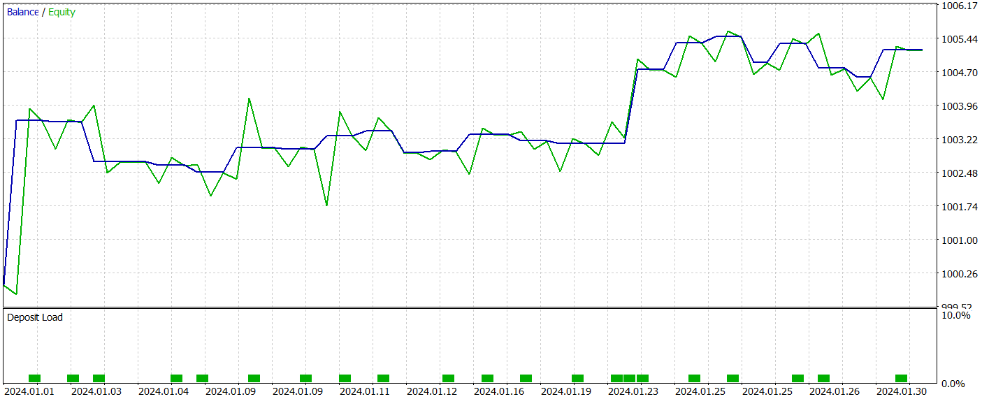

During the test period, the model executed 22 trades, exactly half of which were closed in profit. Notably, the average profit per winning trade was more than twice the average loss per losing trade. The largest profitable trade exceeded the largest loss by a factor of four. As a result, the model achieved a profit factor of 2.63. However, the small number of trades and the short testing period do not allow us to draw any definitive conclusions about the long-term effectiveness of the method. Before using the model in a live environment, it should be trained on a longer historical dataset and subjected to comprehensive testing.
Conclusion
The approaches proposed in the Generalized 3D Referring Expression Segmentation (3D-GRES) method show promising applicability in the domain of trading by enabling deeper analysis of market data. This method can be adapted for segmenting and analyzing multiple market signals, leading to more precise interpretations of complex market conditions, and ultimately improving forecasting accuracy and decision-making.
In the practical part of this article, we implemented our vision of the proposed approaches using MQL5. Our experiments demonstrate the potential of the proposed solutions for use in real-world trading scenarios.
References
Programs used in the article| # | Name | Type | Description |
|---|---|---|---|
| 1 | Research.mq5 | Expert Advisor | EA for collecting examples |
| 2 | ResearchRealORL.mq5 | Expert Advisor | EA for collecting examples using the Real-ORL method |
| 3 | Study.mq5 | Expert Advisor | Model training EA |
| 4 | Test.mq5 | Expert Advisor | Model testing EA |
| 5 | Trajectory.mqh | Class library | System state description structure |
| 6 | NeuroNet.mqh | Class library | A library of classes for creating a neural network |
| 7 | NeuroNet.cl | Library | OpenCL program code library |
Translated from Russian by MetaQuotes Ltd.
Original article: https://www.mql5.com/ru/articles/15997
Warning: All rights to these materials are reserved by MetaQuotes Ltd. Copying or reprinting of these materials in whole or in part is prohibited.
This article was written by a user of the site and reflects their personal views. MetaQuotes Ltd is not responsible for the accuracy of the information presented, nor for any consequences resulting from the use of the solutions, strategies or recommendations described.

- Free trading apps
- Over 8,000 signals for copying
- Economic news for exploring financial markets
You agree to website policy and terms of use