Neural Network in Practice: Straight Line Function

Introduction

I am very glad to welcome everyone and invite you to read a new article about neural networks.

In the previous article "Neural Network in Practice: Least Squares", we looked at how, in very simple cases, we can find an equation that best describes the data set we are using. The equation that was formed in this system was very simple, it used only one variable. We've already shown how to do the calculation, so we'll get straight to the point here. This is because the mathematics used to create an equation based on the values available in the database requires significant knowledge of analytical mathematics and algebraic computation. In addition to this, of course, it is necessary to know what type of data is in the database we are using.

Since this article is meant to be widely educational, I don't want to make things difficult for my readers. If you are really interested in delving into the computations, I suggest you study the materials on this topic. As already mentioned, you will mainly have to study analytical mathematics and algebraic calculus. To make this process less theoretical and tedious, I suggest you start by studying game theory. There you can get acquainted with computations and analysis in a more entertaining form, without the monotonous review of endless computations.

There are many materials on the web on this topic that are well explained and easy to understand. But if your goal is just to look at the code, then you are welcome, since I will not go into the math part in this article. The mathematical question is quite deep and requires understanding every detail and a lot of time. Most readers may not be interested in these aspects.

Therefore, in this article we will just take a quick look at some methods to get a function that could represent our data in the database. I will not go into detail about how to use statistics and probability studies to interpret the results. Let's leave that for those who really want to delve into the mathematical side of the matter. Exploring these questions will be critical to understanding what is involved in studying neural networks. Here we will consider this issue quite calmly.

Creating an equation in general form

First, let's do some calculations. (Again?!). Calm down my dear reader, you don't have to worry about what we're going to do. This time I promise to be kinder. Today we will act differently. Our goal is to create a system capable of generating more general straight line equations. And so as not to leave you completely stunned with the development of the formulas that we will use, we will not go into the mathematical development behind the equations. This is not necessary, since in the previous article we showed what it looks like to develop a mathematical equation based on some fundamental ideas and principles. Here we will just try to understand what these equations actually mean. Of course, we will try to make everything as accessible as possible. Although they may seem confusing at first, I won't let you get confused. Read the article without rushing. See how the whole thing unfolds, because here I will synthesize various studies in mathematics to show you how we can make a neural network learn knowledge based on information contained in a database.

But before we begin, I want to make one thing clear: what we'll see here is for a neural network that won't be receiving any new information into its database. That is, the database is already completely created, and we just want it to generate an equation that best represents what is already in the database. Only later, using other mechanisms, we can filter out the likelihood that new information is related or unrelated to what is already in the database. Such mechanisms usually fall into the field of artificial intelligence. But this is something for another discussion.

Let's now go back to our code example. In this example, we already have two datasets that can be plotted on a two-dimensional plane. That is, only using X and Y coordinates. After a calm analysis of the situation, we can see that the desired equation is relatively easy to construct, since our data can be expressed with some approximation to a probable straight line. Sometimes this is not the case, since the equation may be a curve or a trigonometric function. But let's take it one step at a time. First, we need to deal with simpler cases. Let's start by understanding the following: the equation we want to obtain has the format shown below.

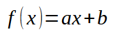
Here the value of the constant < a > represents the slope. The constant < b > is the intersection point. When < b > is zero, the root of the function is also zero. In the previous article we looked at how to calculate this coefficient if < b > is zero. Also, at the end of the same article, we saw how to adjust both values to try to approximate the constants of the equation, thus constructing the linear function shown above. Let's remember again that if we change the value of the constant < b >, the root of the function will also change. Understanding this is important in order to solve the system using polynomials. However, here we will use a method adapted from the previous article.

I think it's clear that trying to find these values by trial and error is what is known in programming as brute force, where all possible values are tried (and this is far from the best way). While this can be done, in most cases the processing time will be very long. In cases like ours, it will simply take a lot of time and effort, but it is entirely doable. However, as the number of variables increases significantly, this process becomes impractical, no matter whether you do it manually or by brute force.

However, even if we decide to use brute force, in the previous article I demonstrated a way to calculate the slope when the constant < b > is zero. This method made it possible to find the angular coefficient relatively simply and quickly, regardless of the volume of data in the database. The only constraint was that the resulting equation had to be a straight line. However, if the constant < b > is not equal to zero, then this calculation will no longer work. This will only give us a rough idea of which direction to move in. We'll look at this later. For now, we'll try to do things based on known functions, such as the one we looked at at the beginning of this topic.

Let us now think about the general case of the solution. Remember that you need to know the type of polynomial you are using. Without this knowledge, finding the equation that best represents the data can be very time-consuming even in the simplest cases. So remember: everything we see next is based on this prior knowledge.

Let's generalize the least squares method to any case. To do this, you need to know the type of polynomial used. We will start with a simple one that generates a straight line. This polynomial can be generalized using the expression shown below.

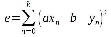
Wait, isn't this the same formula we saw in the previous article? It is! Basically it's the same thing, but now the variable < b > is included in the formula because we no longer assume it is zero. If we expand this sum, we will arrive at something similar to what we did in the previous article. However, for better understanding, when generalizing this calculation we must consider the derivative with respect to both the variable < a > and < b >. This will give us the definition shown below.

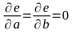
In other words, everything is the same as we did in the previous article. However, this principle is not limited to the equation of a straight line. We can use the same approach in either case. For example, suppose a data set can best be expressed or represented as a parabola. In this case, we need to think about how to find a quadratic equation using the data we have in our database. The last two definitions are transformed into the following.

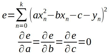
Thus, we will need to develop a new term to find a way to generate an equation, which in this case will be a quadratic equation. That is, we need to find the constants so that a quadratic equation can display everything that is in the database. But, returning to our case where we use the straight line equation, if we now continue the calculation assuming < b > to be non-zero, we first obtain the following equation.

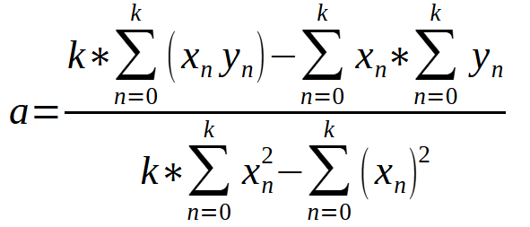
This equation allows us to calculate the value of < a > based on the data contained in our database.

After obtaining the value of the constant < a >, we can use the equation below to find the constant < b >.

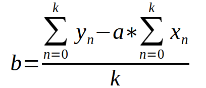
In both cases, the value < k > is the number of points on the graph. Perhaps, looking at the equations alone, you might get confused and think that this is something complicated. Or you might not know how to convert these expressions into code using some programming language. Which would allow way to get the values of constants without doing it manually. This is what we did in the previous article. We will translate this mathematical format into a programming language format, in this case MQL5, but you could use any other language and the results would be the same. Below you can see how these equations will look like in our MQL5 code.

28. //+------------------------------------------------------------------+
29. void Func_01(void)
30. {
31.     int A[]={
32.                   -100, -150,
33.                    -80,  -50,
34.                     30,   80,
35.                    100,  120
36.             };
37. 
38.     int vx, vy;
39.     uint k;
40.     double ly, err, dx, dy, dxy, dx2, a, b;
41.     string s0 = "";
42. 
43.     canvas.LineVertical(global.x, global.y - _SizeLine, global.y + _SizeLine, ColorToARGB(clrRoyalBlue, 255));
44.     canvas.LineHorizontal(global.x - _SizeLine, global.x + _SizeLine, global.y, ColorToARGB(clrRoyalBlue, 255));
45. 
46.     err = dx = dy = dxy = dx2 = 0;
47.     k = 0;    
48.     for (uint c0 = 0, c1 = 0; c1 < A.Size(); c0++, k++)
49.     {
50.         vx = A[c1++];
51.         vy = A[c1++];
52.         dx += vx;
53.         dy += vy;
54.         dxy += (vx * vy);
55.         dx2 += MathPow(vx, 2);
56.         canvas.FillCircle(global.x + vx, global.y - vy, 5, ColorToARGB(clrRed, 255));
57.         ly = vy - (vx * -MathTan(_ToRadians(global.Angle))) - global.Const_B;
58.         s0 += StringFormat("%.4f || ", MathAbs(ly));
59.         canvas.LineVertical(global.x + vx, global.y - vy, global.y + (int)(ly - vy), ColorToARGB(clrPurple));
60.         err += MathPow(ly, 2);
61.     }
62.     a = ((k * dxy) - (dx * dy)) / ((k * dx2) - MathPow(dx, 2));
63.     b = (dy - (a * dx)) / k;
64.     PlotText(3, StringFormat("Error: %.8f", err));
65.     PlotText(4, s0);
66.     PlotText(5, StringFormat("f(x) = %.4fx %c %.4f", a, (b < 0 ? '-' : '+'), MathAbs(b)));
67. }
68. //+------------------------------------------------------------------+

Let's figure out what's going on in this fragment. In lines 46 and 47, we initialize all variables to zero. This is because we want to explicitly show that they start at zero, although we could skip this declaration since the compiler usually initializes variables to zero implicitly. In line 52, we calculate the sum of all X values, and in line 53 we calculate the sum of Y values. In line 54, we calculate the sum of the product of the X and Y values. And finally, in line 55, we calculate the sum of the squares of the X values.

All of these calculations are used in the formulas we've already looked at before. In other words, doing the calculations is much easier than it seems. All the above calculations are used in the formulas we have previously considered. So it is much simpler this time.

Now we need to calculate the values of the constants used in the equation of a straight line. For this, we use line 62, where we calculate the slope value, and line 63 where we find the intercept value. Have you noticed how easy it is to turn a mathematical formula into a calculation that our program can perform? There are people who claim to understand mathematics but cannot translate it into programming terms. In my opinion, these people are deceiving themselves, because writing a mathematical formula in code is as easy as reading it. Of course, if we don't understand the formula, we can't explain to a computer, which is just a giant calculator, how to do the calculation.

Now, we plot the resulting equation. This is done in line 66. This allows us to manually visualize whether the calculated values are the most appropriate for the given data set. In the GIF below, you can see the result of running our program with the values specified in matrix A present in line 31.

See how the error values change as we try to find the ideal point. Compare the equation of a straight line shown as ideal with the equation of the line we are trying to plot using the arrows. We do not get a very accurate setting, but we have a value very close to the ideal. Understanding this is important because we will soon be studying this same property, but in a different way.

Now you might be wondering: is there a way to get closer to the calculated value? Yes, dear reader, there is. To do this, you simply need to change a value in the program as shown in the code below.

void NewAngle(const char direct, const char updow, const double step = 0.1)

The value to be changed is the step argument. Here we use a step of 0.1 as you can see in the code, but you can use a smaller or larger value. If you use a smaller value, the program will take longer to reach the calculated values, but the error accuracy will be higher due to less variance. Remember that one outweighs the other: there is no 100% perfect solution, but there is an ideal balance point.

Once we have code that can calculate the line equation, we can freely change the values in matrix A to create any conditions or knowledge base. You may just need to change the type of variables you use. Here we are using integers, but if you want to use floating data types like double or float, just change the type, the calculation will not change. This is necessary in order to obtain the equation of the line. However, if the data in the database is best represented by, say, a quadratic equation, we will have to modify the calculations to find the best system of constants to represent our database, as discussed above. It all depends on the context; there is no 100% effective solution for all possible and conceivable cases.

But you might think that this is the only way to calculate the equation of a straight line. If you thought exactly this way, then your knowledge is still insufficient. To show another way to obtain the same values we have been looking at in this topic, we will study a new section, dividing the concepts accordingly. This section will be an introduction to what we will see in the next article.

Pseudoinverse

Until now, everything seemed very complicated and difficult to implement in code. This is because each required change must be properly implemented in the generated code. However, there is a nicer way to write code for this situation, in which the variables are constantly changing. At least that's what I believe. When it comes to writing code where the number of variables changes frequently, I prefer to move from scalar to matrix calculations. Matrix operations allow us to take into account any factors without having to create a lot of time variables. I know many of you find writing code for matrix factorization very difficult and often use libraries that perform this factorization without understanding how it works. This can make you dependent on these libraries because you don't understand how the calculations are done.

Some time ago I wrote two articles to introduce matrix factorization. In those articles, we looked at the most basic elements we should know in order to create code that performs matrix factorization operations. Many problems are solved more easily and quickly if you use matrices for calculations.

Articles: "Matrix Factorization: The Basics" and "Matrix Factorization: A more practical modeling". If you want to learn more about this topic, I recommend you read and test in practice what is presented in these articles. Of course, they only cover the basics, but if you understand their content, you can understand what we will be doing in this section.

Here we will use matrices to find the values obtained in the previous topic. To understand what we are going to do, we need to know how matrices are added up. I don't mean programming, since programming these calculations is the easy part. I mean that you should have at least a basic knowledge of how to perform computations using matrices. I will not go into detail on how to do these calculations, as I assume that you have some knowledge in this area. You do not need to be an expert. Knowing the basics will be enough for what we are going to do.

Let's now go back to how to find the equation of a straight line, given that we have a database and we want to save the database contents as a mathematical equation. At first glance, it seems very difficult, as if only a genius could accomplish this. But no, we will do the same as in the previous topic. Just a little differently.

Let's start with the basics. The error equation is shown in the figure below.

This is the scalar form of the equation. However, we can write the same equation in matrix form as shown below.

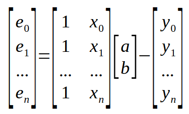
This matrix representation is exactly what is shown in the previous picture, without any additions. But we can simplify this matrix representation even further. We do it as follows:

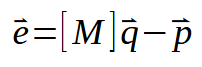
I know this representation may seem very complicated. Yet it represents exactly what a scalar computation would do. However, this more compact form of matrix factorization will allow us to better understand how the calculations will be performed, since we will need to write fewer elements in the formula. Here we indicate that the vector < e > is equal to the matrix < M >, which contains the x values, multiplied by the vector < q >, which contains the constants we are looking for. These include the angular coefficient and the intersection point. We then subtract the vector < p >, which represents the values of the matrix containing the y values.

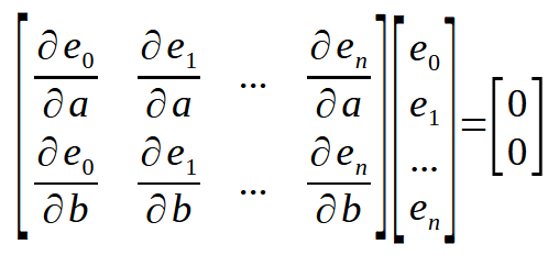
Now I want to remind you of the following: we are looking for the derivative of the constants <a> and <b> with respect to the error, which we can easily calculate. Now we have the location of the points that we will use in the calculation. Therefore, if we represent it in matrix form, we can get the following.

Here is a small detail:

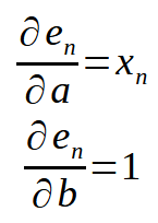
If we remember that < n > represents the array index in our code, the above equation can be rewritten as shown below.

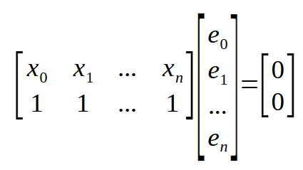
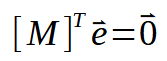
Okay, now we have something really interesting. If you look at the matrices above, you can see that we show the same result here. It also appears in other places, only this matrix is transposed, and this makes the formula even more compact. Look at the image below.

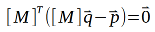
The next step is to make some substitutions in the data we already have. Thus, we obtain the following formulation.

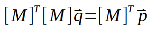
Let's now develop this calculation or formula (you can call it whatever you want) shown above. This brings us to the following:

Now if we invert the transposed matrix, we get something like this:

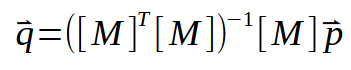
This result is actually a very nice and interesting factorization, so much so that the person who created it actually deserved the Nobel Prize in Mathematics in 2020. This formulation is known as the Moore-Penrose pseudoinverse, after its creators. It gives us exactly what we are looking for, which is the angular coefficient and intercept values. And both will be inside the vector < q >. This type of calculation can be implemented in a variety of different programs, many of which are designed exclusively for working with calculations. For example, using SCILab, you can use the program shown below. It will calculate the values of the slope and the intersection point.

clc;
clear;
clf;

x=[-100; -80; 30; 100];
y=[-150; -50; 80; 120];

A = [ones(x), x];

plot(x, y, 'ro');
zoom_rect([-150, -180, 180, 180]);
xgrid;

x = pinv(A) * y;
b = x(1);
a = x(2);

x =[-120:1:120];
y = a * x + b;

plot(x, y, 'b-');

The result of execution can be seen just below:

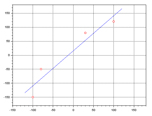
The red dots indicate the location of the same points as in the MQL5 program. The blue line shows the result of the line equation obtained using the pseudoinverse. The same can be done using MATLAB, as well as other programs such as Excel. This is explained by the great usefulness of this pseudoinverse in various fields.

To give you an idea of how interesting this pseudoinverse is, we can just slightly change the vectors used, as well as the matrices of the equation. You can solve polynomials of any kind, and quite effectively.

Final considerations

Since the pseudoinverse is a factorization that must be done using matrices, I will not show in this article what the program for finding the constants < a > and < b > would look like. This is because we will need to consider certain explanations for you to really understand what is going on. It's not just about presenting the code itself. Matrix operations require much more attention due to the peculiarities of their processing. When performed manually, the operations are relatively simple. However, doing this in code is a completely different story. Even in those articles where we talk about how to use factorization in matrices, what they do there is not general, they are very specific. But for our purposes we need a more general code. Otherwise, the pseudoinverse will not be computed correctly.