Neural Networks Made Easy (Part 88): Time-Series Dense Encoder (TiDE)

MetaTrader 5 — Trading systems | 20 September 2024, 16:04

3 523

Dmitriy Gizlyk

Introduction

Probably all known neural network architectures have been studied in terms of their ability to solve time series forecasting problems, including recurrent, convolutional and graph models. The most notable results are demonstrated by models based on the Transformer architecture. Several such algorithms were also presented in this series of articles. However, recent research has shown that Transformer-based architectures might be less powerful than expected. On some time series forecasting benchmarks, simple linear models can show comparable or even better performance. Unfortunately, however, such linear models have shortcomings because they are not suitable for modeling nonlinear relationships between a sequence of time series and time-independent covariates.

Further research in the field of time series analysis and forecasting split into two directions. Some see Transformer potential that has not been fully realized and are working to improve the efficiency of such architectures. Others try to minimize the shortcomings of linear models. The paper entitled "Long-term Forecasting with TiDE: Time-series Dense Encoder" refers to the second direction. This paper proposes a simple and efficient deep learning architecture for time series forecasting that achieves better performance than existing deep learning models on popular benchmarks. The presented model based on a Multilayer Perceptron (MLP) is surprisingly simple and does not include Self-Attention mechanisms, recurrent or convolutional layers. Therefore, it has linear computational scalability with respect to context length and prediction horizon, unlike many Transformer-based solutions.

The Time-series Dense Encoder (TiDE) model uses MLP to encode the past time series together with covariates and to decode the forecast time series together with future covariates.

The authors of the method analyze a simplified linear model TiDE and show that this linear model can achieve near-optimal error in linear dynamic systems (LDS), when the LDS design matrix has a maximum singular value different from 1. They test this empirically on simulated data: the linear model outperforms both LSTMs and Tarnsformers.

On popular real-world time series forecasting benchmarks, TiDE achieves better or similar results compared to previous baseline neural network models. At the same time, TiDE is 5x faster in production and over 10x faster in training than the best Transformer-based models.

1. TiDE Algorithm

The TiDE (Time-series Dense Encoder) model is a simple and efficient MLP-based architecture for long-term time series forecasting. The authors of the algorithm add nonlinearity in the form of an MLP so that they can handle past data and covariates. The model is applied to independent data channels, that is, the model input is the past and covariates of one time series at a time. In this case, the model weights are trained globally using the entire data set, i.e. they are the same for all independent channels.

The key component of the model is the MLP closed-loop block. The MLP has one hidden layer and ReLU activation. It also has a skip connection that is completely linear. The authors of the method use Dropout on the linear layer that maps the hidden layer to the output, and also use the normalization layer on the output.

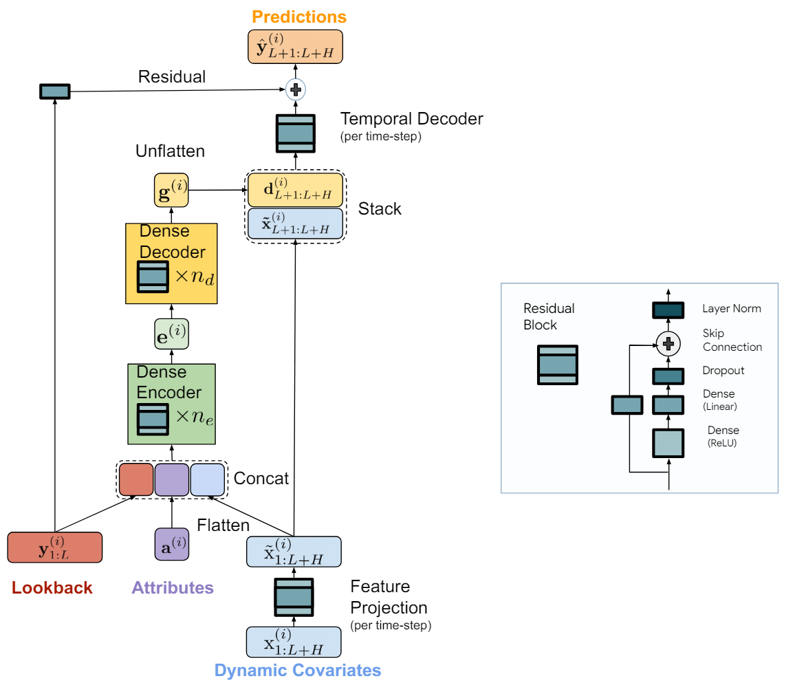
The TiDE model is logically divided into encoding and decoding sections. The encoding section contains a feature projection step followed by a dense MLP encoder. The decoding section consists of a dense decoder followed by a temporal decoder. Dense encoder and dense decoder can be combined into one block. However, the authors of the method separate them because they use different sizes of hidden layers in the two blocks. Also, the last layer of the decoder block is unique: its output size must match the planning horizon.

The goal of the coding step is to map the history and covariates of the time series into a dense feature representation. Encoding in the TiDE model has two key steps.

Initially, a closed-loop block is used to map the covariates at each time step (both in the historical context and in the forecast horizon) into a lower-dimensional projection.

We then pool and smooth all past and future projected covariates, combining them with the static attributes and the past time series. After that, we map them into an embedding using a dense encoder that contains multiple closed-loop blocks. Decoding in the TiDE model maps encoded latent representations into future forecast values of the time series. It also includes two operations: dense decoder and temporal decoder.

A dense decoder is a stack of several closed-loop blocks similar to the encoder blocks. It takes the output of the encoder as input and maps it into a vector of predicted states.

The model output uses a temporal decoder to generate final predictions. A temporal decoder is the same closed-loop block that maps the decoded vector to the t-th time step of the forecast horizon, combined with the projected covariates of the forecast period. This operation adds a connection from the future covariates to the prediction of the time series. This can be useful if some covariates have a strong direct effect on the actual value at a particular time step. For example, the news background on individual calendar days.

To the values of the temporal decoder, we add the values of the global residual connection, which linearly maps the past of the analyzed time series to the planning horizon vector. This ensures that a purely linear model is always a subclass of the TiDE model.

The author's visualization of the method is presented below.

The model is trained using mini-batch gradient descent. The authors of the method use MSE as the loss function. Each epoch includes all pairs of past and forecast horizon that can be constructed from the training period. Thus, two mini batches can have overlapping time points.

2. Implementing in MQL5

We have considered the theoretical aspects of the TiDE algorithm. Now we can move on to the practical implementation of these approaches using MQL5.

As already mentioned above, the main "building block" of the TiDE method we are considering is a closed-loop block. In this block, the authors of the method use fully connected layers. However, note that each such block in the model is applied to a separate independent channel. In this case, the trainable parameters of the block are trained globally and are the same for all channels of the analyzed multidimensional time series.

Of course, in our implementation we would like to implement parallel computing for all independent channels of the multidimensional time series we are analyzing. In similar cases we previously used convolutional layers with multiple convolution filters. The window size of such a convolutional layer is equal to its stride and corresponds to the data volume of one channel. I think it is obvious that it is equal to the depth of the analyzed time series history.

Since we've come to the point of using convolutional layers, let's recall the closed-loop convolutional block, which we created when implementing the CCMR method. If you read attentively, you may notice the difference: the CCMR implementation used normalization layers. However, in the context of this article, I decided to ignore this difference in the block architecture. Therefore, we will use the previously created CResidualConv block to build a new model.

So, we have the basic "building block" for the proposed TiDE algorithm. Now we need to assemble the entire algorithm from these blocks.

2.1 TiDE Algorithm Class

Let's implement the proposed approaches in the new CNeuronTiDEOCL class, inheriting it from the neural layer base class CNeuronBaseOCL. The architecture of our new class requires 4 key parameters for which we will declare local variables:

iHistory – the depth of the analyzed time series history
iForecast – time series forecasting horizon
iVariables – the number of analyzed variables (channels)
iFeatures – the number of covariates in the time series

class CNeuronTiDEOCL :  public CNeuronBaseOCL
  {
protected:
   uint              iHistory;
   uint              iForecast;
   uint              iVariables;
   uint              iFeatures;
   //---
   CResidualConv     acEncoderDecoder[];
   CNeuronConvOCL    cGlobalResidual;
   CResidualConv     acFeatureProjection[2];
   CResidualConv     cTemporalDecoder;
   //---
   CNeuronBaseOCL    cHistoryInput;
   CNeuronBaseOCL    cFeatureInput;
   CNeuronBaseOCL    cEncoderInput;
   CNeuronBaseOCL    cTemporalDecoderInput;
   //---
   virtual bool      feedForward(CNeuronBaseOCL *NeuronOCL, CBufferFloat *SecondInput);
   virtual bool      updateInputWeights(CNeuronBaseOCL *NeuronOCL, CBufferFloat *SecondInput);
   virtual bool      calcInputGradients(CNeuronBaseOCL *NeuronOCL, CBufferFloat *SecondInput, 
                                        CBufferFloat *SecondGradient, 
                                        ENUM_ACTIVATION SecondActivation = None);

public:
                     CNeuronTiDEOCL(void) {};
                    ~CNeuronTiDEOCL(void) {};
   //---
   virtual bool      Init(uint numOutputs, uint myIndex, COpenCLMy *open_cl, 
                          uint history, uint forecast, uint variables, uint features, 
                          uint &encoder_decoder[], ENUM_OPTIMIZATION optimization_type, 
                          uint batch);
   //---
   virtual bool      Save(int const file_handle);
   virtual bool      Load(int const file_handle);
   //---
   virtual int       Type(void)        const                      {  return defNeuronTiDEOCL; }
   virtual void      SetOpenCL(COpenCLMy *obj);
   //---
   virtual bool      WeightsUpdate(CNeuronBaseOCL *source, float tau);
  };

As you can see, the variables do not include the number of blocks in either the Encoder or the Decoder of the model. In our implementation, we combined the Encoder and Decoder into an array of acEncoderDecoder[] blocks. The size of this array will point to the total number of closed-loop blocks used to encode historical data and decode the predicted time series values.

In addition, we divided the projection of the time series covariates into 2 blocks (acFeatureProjection[2]). In one of them, we will generate a projection of covariates to encode historical data; in the second one – to decode predicted values.

We will also add a temporal decoder block cTemporalDecoder. For the global residual connection, we will use the cGlobalResidual convolutional layer.

Additionally, we declare 4 local fully connected layers for writing intermediate values. The specific purpose of each layer will be explained during the implementation process.

We have declared all objects in our class as static, which allows us to leave the class constructor and destructor "empty".

The set of overridable methods is quite standard. As always, let's begin by considering the class object initializing method CNeuronTiDEOCL::Init.

bool CNeuronTiDEOCL::Init(uint numOutputs, uint myIndex, COpenCLMy *open_cl, uint history, 
                          uint forecast, uint variables, uint features, uint &encoder_decoder[],
                          ENUM_OPTIMIZATION optimization_type, uint batch)
  {
   if(!CNeuronBaseOCL::Init(numOutputs, myIndex, open_cl, forecast * variables, 
                            optimization_type, batch))
      return false;

In the parameters, the method receives all the necessary information to implement the required architecture. In the body of the method, we first call the same method of the parent class, which implements the minimum necessary control of the received parameters and initialization of the inherited objects.

After the parent class initialization method operations are successfully executed, we save the values of the key constants.

   iHistory = MathMax(history, 1);
   iForecast = forecast;
   iVariables = variables;
   iFeatures = MathMax(features, 1);

Then we move on to initializing internal objects. First we initialize the covariate projection blocks.

   if(!acFeatureProjection[0].Init(0, 0, OpenCL, iFeatures, iHistory * iVariables, 1, 
                                                                 optimization, iBatch))
      return false;
   if(!acFeatureProjection[1].Init(0, 1, OpenCL, iFeatures, iForecast * iVariables, 1, 
                                                                 optimization, iBatch))
      return false;

Please note that in our experiment, we do not use any a priori knowledge about the covariates of the analyzed time series. Instead, we project the time harmonics of the timestamp onto the sequence. In doing so, we generate our own projections for each channel (variable) of the analyzed multidimensional time channel.

We obtain the dimensions of the hidden layers of the dense encoder and decoder in the form of the encoder_decoder[] array. The array size indicates the total number of closed-loop blocks in the encoder and decoder. The value of the array elements indicates the dimension of the corresponding block. Remember that the input to the encoder is a concatenated vector of historical time series data with a projection of covariates. At the output of the decoder we need to obtain a vector corresponding to the forecast horizon. To enable the latter, we add another block at the decoder output of the required size.

   int total = ArraySize(encoder_decoder);
   if(ArrayResize(acEncoderDecoder, total + 1) < total + 1)
      return false;
   if(total == 0)
     {
      if(!acEncoderDecoder[0].Init(0, 2, OpenCL, 2 * iHistory, iForecast, iVariables,
                                                                 optimization, iBatch))
         return false;
     }
   else
     {
      if(!acEncoderDecoder[0].Init(0, 2, OpenCL, 2 * iHistory, encoder_decoder[0], iVariables, 
                                                                          optimization, iBatch))
         return false;
      for(int i = 1; i < total; i++)
         if(!acEncoderDecoder[i].Init(0, i + 2, OpenCL, encoder_decoder[i - 1], 
                                          encoder_decoder[i], iVariables, optimization, iBatch))
            return false;
      if(!acEncoderDecoder[total].Init(0, total + 2, OpenCL, encoder_decoder[total - 1],
                                                   iForecast, iVariables, optimization, iBatch))
         return false;
     }

Next we initialize the temporal decoder block and the global feedback layer.

   if(!cGlobalResidual.Init(0, total + 3, OpenCL, iHistory, iHistory, iForecast, iVariables, 
                                                                        optimization, iBatch))
      return false;
   cGlobalResidual.SetActivationFunction(TANH);
   if(!cTemporalDecoder.Init(0, total + 4, OpenCL, 2 * iForecast, iForecast, iVariables, 
                                                                        optimization, iBatch))
      return false;

Pay attention to the following two points:

The temporal decoder receives as input a concatenated matrix of predicted time series values and projections of prediction covariates. At the output of the block, we receive adjusted predicted time series values.
At the output of each CResidualConv block data is normalized: the average value of each channel is equal to "0" and the variance is equal to "1". To bring the data of the global closed-loop block into a comparable form, we will use the hyperbolic tangent (tanh) as the activation function for the cGlobalResidual layer.

In the next step, we initialize the auxiliary objects for storing intermediate data. We will save the historical data of the analyzed multivariate time series and the covariates obtained from the external program in cHistoryInput and cFeatureInput, respectively.

   if(!cHistoryInput.Init(0, total + 5, OpenCL, iHistory * iVariables, optimization, iBatch))
      return false;
   if(!cFeatureInput.Init(0, total + 6, OpenCL, iFeatures, optimization, iBatch))
      return false;

We write the concatenated matrix of historical data and covariate projections in cEncoderInput.

   if(!cEncoderInput.Init(0, total + 7, OpenCL, 2 * iHistory * iVariables, optimization,iBatch))
      return false;

The output of the dense decoder will be concatenated with the predicted value covariates and written to cTemporalDecoderInput.

   if(!cTemporalDecoderInput.Init(0, total + 8, OpenCL, 2 * iForecast * iVariables, 
                                                                         optimization, iBatch))
      return false;

At the end of the class object initialization method, we will swap of data buffers to eliminate extra copying of error gradients between the data buffers of individual elements of our class.

   if(cGlobalResidual.getGradient() != Gradient)
      if(!cGlobalResidual.SetGradient(Gradient))
         return false;
   if(cTemporalDecoder.getGradient() != getGradient())
      if(!cTemporalDecoder.SetGradient(Gradient))
         return false;
//---
   return true;
  }

After completing class instance initialization, we move on to constructing the feed-forward algorithm, which is described in the CNeuronTiDEOCL::feedForward method. In the method parameters we receive pointers to 2 objects containing input data. This is historical multivariate time series data in the form of a results buffer from the previous neural layer and covariates represented as separate data buffers.

bool CNeuronTiDEOCL::feedForward(CNeuronBaseOCL *NeuronOCL, CBufferFloat *SecondInput)
  {
   if(!NeuronOCL || !SecondInput)
      return false;

In the method body, we immediately check if the received pointers are relevant.

Next, we need to copy the received input data into internal objects. However, instead of transferring the entire amount of information, we will only check the pointers to the data buffers and copy them if necessary.

   if(cHistoryInput.getOutputIndex() != NeuronOCL.getOutputIndex())
     {
      CBufferFloat *temp = cHistoryInput.getOutput();
      if(!temp.BufferSet(NeuronOCL.getOutputIndex()))
         return false;
     }
   if(cFeatureInput.getOutputIndex() != SecondInput.GetIndex())
     {
      CBufferFloat *temp = cFeatureInput.getOutput();
      if(!temp.BufferSet(SecondInput.GetIndex()))
         return false;
     }

After carrying out the preparatory work, we project the historical data into the dimension of forecast values. This is a kind of autoregressive model.

   if(!cGlobalResidual.FeedForward(NeuronOCL))
      return false;

We generate projections of covariates to historical and predicted values.

   if(!acFeatureProjection[0].FeedForward(NeuronOCL))
      return false;
   if(!acFeatureProjection[1].FeedForward(cFeatureInput.AsObject()))
      return false;

We then concatenate the historical data with the corresponding covariate projection matrix.

   if(!Concat(NeuronOCL.getOutput(), acFeatureProjection[0].getOutput(), 
              cEncoderInput.getOutput(), iHistory, iHistory, iVariables))
      return false;

Create a loop of operations of the dense encoder and decoder block.

   uint total = acEncoderDecoder.Size();
   CNeuronBaseOCL *prev = cEncoderInput.AsObject();
   for(uint i = 0; i < total; i++)
     {
      if(!acEncoderDecoder[i].FeedForward(prev))
         return false;
      prev = acEncoderDecoder[i].AsObject();
     }

We concatenate the decoder's output with the projection of the predicted values' covariates.

   if(!Concat(prev.getOutput(), acFeatureProjection[1].getOutput(), 
              cTemporalDecoderInput.getOutput(), iForecast, iForecast, iVariables))
      return false;

The concatenated matrix is fed into the time decoder block.

   if(!cTemporalDecoder.FeedForward(cTemporalDecoderInput.AsObject()))
      return false;

At the end of the feed-forward operations, we sum the results of the 2 data streams and normalize the resulting result across independent channels.

   if(!SumAndNormilize(cGlobalResidual.getOutput(), cTemporalDecoder.getOutput(), Output, 
                                                                         iForecast, true))
      return false;
//---
   return true;
  }

The feed-forward pass is followed by a backpropagation pass, which consists of 2 layers. First, we distribute the error gradient between all internal objects and external inputs according to their influence on the final result in the CNeuronTiDEOCL::calcInputGradients method. In the parameters, the method receives pointers to objects for writing the error gradients of the input data.

bool CNeuronTiDEOCL::calcInputGradients(CNeuronBaseOCL *NeuronOCL, CBufferFloat *SecondInput, 
                          CBufferFloat *SecondGradient, ENUM_ACTIVATION SecondActivation = -1)
  {
   if(!cTemporalDecoderInput.calcHiddenGradients(cTemporalDecoder.AsObject()))
      return false;

Since we use the swapping of data buffers, there is no need to copy data from our class's error gradients into the relevant buffers of nested objects. So, we call the error gradient distribution methods of our nested blocks in the reverse order.

First, we propagate the error gradient through the temporal decoder block. We distribute the operation result across the dense decoder and the projection of the predicted time series covariates.

   int total = (int)acEncoderDecoder.Size();
   if(!DeConcat(acEncoderDecoder[total - 1].getGradient(), acFeatureProjection[1].getGradient(),
                cTemporalDecoderInput.getGradient(), iForecast, iForecast, iVariables))
      return false;

After that, we distribute the error gradient across the dense encoder and decoder block.

   for(int i = total - 2; i >= 0; i--)
      if(!acEncoderDecoder[i].calcHiddenGradients(acEncoderDecoder[i + 1].AsObject()))
         return false;
   if(!cEncoderInput.calcHiddenGradients(acEncoderDecoder[0].AsObject()))
      return false;

The error gradient at the level of the dense encoder's input data is distributed across historical data of the multivariate time series and the corresponding covariates.

   if(!DeConcat(cHistoryInput.getGradient(), acFeatureProjection[0].getGradient(),
                cEncoderInput.getGradient(), iHistory, iHistory, iVariables))
      return false;

Next, we adjust the error gradient of the global feedback layer by the derivative of the activation function.

   if(cGlobalResidual.Activation() != None)
     {
      if(!DeActivation(cGlobalResidual.getOutput(), cGlobalResidual.getGradient(),
                       cGlobalResidual.getGradient(), cGlobalResidual.Activation()))
         return false;
     }

Lower the error gradient to the input data level.

   if(!NeuronOCL.calcHiddenGradients(cGlobalResidual.AsObject()))
      return false;

Here we will also adjust the error gradient of the second data stream by the derivative of the activation function of the previous layer.

   if(NeuronOCL.Activation()!=None)
      if(!DeActivation(cHistoryInput.getOutput(),cHistoryInput.getGradient(),
                       cHistoryInput.getGradient(),SecondActivation))
        return false;

After that we sum the error gradients from both data streams.

   if(!SumAndNormilize(NeuronOCL.getGradient(), cHistoryInput.getGradient(),
                       NeuronOCL.getGradient(), iHistory, false, 0, 0, 0, 1))
      return false;

At this stage, we have propagated the error gradient to the historical data level of the multivariate time series. Now we need to propagate the error gradient to the covariates.

It should be said here that within the framework of the experiment we are conducting, this process is unnecessary. For covariates, we use timestamp harmonics that are given by the formula. This formula is not adjusted during the learning process. However, we create a process of propagating the gradient to the covariate level with a "future-proofing" in mind. In subsequent experiments, we can try different models of learning time series covariates.

So, we propagate the error gradient from the covariates of historical data. The obtained values are transferred to the buffer of covariate gradients.

   if(!cFeatureInput.calcHiddenGradients(acFeatureProjection[0].AsObject()))
      return false;
   if(!SumAndNormilize(cFeatureInput.getGradient(), cFeatureInput.getGradient(), SecondGradient,
                                                               iFeatures, false, 0, 0, 0, 0.5f))
      return false;

After that we obtain the gradients of the covariates of the predicted values and sum the result of the 2 data streams.

   if(!cFeatureInput.calcHiddenGradients(acFeatureProjection[1].AsObject()))
      return false;
   if(!SumAndNormilize(SecondGradient, cFeatureInput.getGradient(), SecondGradient, iFeatures, 
                                                                          false, 0, 0, 0, 1.0f))
      return false;

If necessary, we adjust the error gradient for the derivative of the activation function.

   if(SecondActivation!=None)
      if(!DeActivation(SecondInput,SecondGradient,SecondGradient,SecondActivation))
        return false;
//---
   return true;
  }

The second step of the backpropagation pass is to adjust the model's training parameters. This functionality is implemented in the CNeuronTiDEOCL::updateInputWeights method. The method algorithm is quite simple. We simply call the corresponding method of all internal objects that have trainable parameters one by one.

bool CNeuronTiDEOCL::updateInputWeights(CNeuronBaseOCL *NeuronOCL, CBufferFloat *SecondInput)
  {
//---
   if(!cGlobalResidual.UpdateInputWeights(cHistoryInput.AsObject()))
      return false;
   if(!acFeatureProjection[0].UpdateInputWeights(cHistoryInput.AsObject()))
      return false;
   if(!acFeatureProjection[1].UpdateInputWeights(cFeatureInput.AsObject()))
      return false;
//---
   uint total = acEncoderDecoder.Size();
   CNeuronBaseOCL *prev = cEncoderInput.AsObject();
   for(uint i = 0; i < total; i++)
     {
      if(!acEncoderDecoder[i].UpdateInputWeights(prev))
         return false;
      prev = acEncoderDecoder[i].AsObject();
     }
//---
   if(!cTemporalDecoder.UpdateInputWeights(cTemporalDecoderInput.AsObject()))
      return false;
//---
   return true;
  }

I would like to say a few words about the file operation methods. To save disk space, we only save key constants and objects with trainable parameters.

bool CNeuronTiDEOCL::Save(const int file_handle)
  {
   if(!CNeuronBaseOCL::Save(file_handle))
      return false;
//---
   if(FileWriteInteger(file_handle, (int)iHistory, INT_VALUE) < INT_VALUE)
      return false;
   if(FileWriteInteger(file_handle, (int)iForecast, INT_VALUE) < INT_VALUE)
      return false;
   if(FileWriteInteger(file_handle, (int)iVariables, INT_VALUE) < INT_VALUE)
      return false;
   if(FileWriteInteger(file_handle, (int)iFeatures, INT_VALUE) < INT_VALUE)
      return false;
//---
   uint total = acEncoderDecoder.Size();
   if(FileWriteInteger(file_handle, (int)total, INT_VALUE) < INT_VALUE)
      return false;
   for(uint i = 0; i < total; i++)
      if(!acEncoderDecoder[i].Save(file_handle))
         return false;
   if(!cGlobalResidual.Save(file_handle))
      return false;
   for(int i = 0; i < 2; i++)
      if(!acFeatureProjection[i].Save(file_handle))
         return false;
   if(!cTemporalDecoder.Save(file_handle))
      return false;
//---
   return true;
  }

However, this leads to some complication in the algorithm of the data loading method CNeuronTiDEOCL::Load. As before, the method receives in parameters a file handle for loading data. First we load the parent object data.

bool CNeuronTiDEOCL::Load(const int file_handle)
  {
   if(!CNeuronBaseOCL::Load(file_handle))
      return false;

Then we read the values of the key constants.

   if(FileIsEnding(file_handle))
      return false;
   iHistory = (uint)FileReadInteger(file_handle);
   if(FileIsEnding(file_handle))
      return false;
   iForecast = (uint)FileReadInteger(file_handle);
   if(FileIsEnding(file_handle))
      return false;
   iVariables = (uint)FileReadInteger(file_handle);
   if(FileIsEnding(file_handle))
      return false;
   iFeatures = (uint)FileReadInteger(file_handle);
   if(FileIsEnding(file_handle))
      return false;

Next we need to load the data from the dense encoder and decoder block. Here we encounter the first nuance. We read the block stack size from the data file. It may be either larger or smaller than the current size of the acEncoderDecoder array. If necessary, we adjust the array size.

   int total = FileReadInteger(file_handle);
   int prev_size = (int)acEncoderDecoder.Size();
   if(prev_size != total)
      if(ArrayResize(acEncoderDecoder, total) < total)
         return false;

Next we run a loop and read the block data from the file. However, before calling the method for loading the data of the added array elements, we need to initialize them. This does not apply to previously created objects, as they were initialized in earlier steps.

   for(int i = 0; i < total; i++)
     {
      if(i >= prev_size)
         if(!acEncoderDecoder[i].Init(0, i + 2, OpenCL, 1, 1, 1, ADAM, 1))
            return false;
      if(!LoadInsideLayer(file_handle, acEncoderDecoder[i].AsObject()))
         return false;
     }

Next, we load the global residual, covariate projection, and temporal decoder objects. Everything is straightforward here.

   if(!LoadInsideLayer(file_handle, cGlobalResidual.AsObject()))
      return false;
   for(int i = 0; i < 2; i++)
      if(!LoadInsideLayer(file_handle, acFeatureProjection[i].AsObject()))
         return false;
   if(!LoadInsideLayer(file_handle, cTemporalDecoder.AsObject()))
      return false;

At this point, we have loaded all the saved data. But we still have auxiliary objects, which we initialize similarly to the class initialization algorithm.

   if(!cHistoryInput.Init(0, total + 5, OpenCL, iHistory * iVariables, optimization, iBatch))
      return false;
   if(!cFeatureInput.Init(0, total + 6, OpenCL, iFeatures, optimization, iBatch))
      return false;
   if(!cEncoderInput.Init(0, total + 7, OpenCL, 2 * iHistory * iVariables, optimization,iBatch))
      return false;
   if(!cTemporalDecoderInput.Init(0, total + 8, OpenCL, 2 * iForecast * iVariables,optimization,
                                                                                        iBatch))
      return false;

If necessary, swap data buffers.

   if(cGlobalResidual.getGradient() != Gradient)
      if(!cGlobalResidual.SetGradient(Gradient))
         return false;
   if(cTemporalDecoder.getGradient() != getGradient())
      if(!cTemporalDecoder.SetGradient(Gradient))
         return false;
//---
   return true;
  }

The full code of all methods of this new class is available in the attachment below. There you will also find auxiliary methods of the class that were not discussed in this article. Their algorithm is quite simple, so you can study them on your own. Let's move on to considering the model training architecture.

2.2 Model architecture for training

As you may have guessed, the new TiDE method class has been added to the environmental state Encoder architecture. We did the same for all the previously considered algorithms that predict future states of a time series. As you remember, we describe the Encoder architecture in the CreateEncoderDescriptions method. In the method parameters, we receive a pointer to a dynamic array object for writing the architecture of the model we are creating.

bool CreateEncoderDescriptions(CArrayObj *encoder)
  {
//---
   CLayerDescription *descr;
//---
   if(!encoder)
     {
      encoder = new CArrayObj();
      if(!encoder)
         return false;
     }

In the body of the method, we check the received pointer and, if necessary, create a new instance of the dynamic array object.

We feed the model with raw historical data received from the terminal.

//--- Encoder
   encoder.Clear();
//--- Input layer
   if(!(descr = new CLayerDescription()))
      return false;
   descr.type = defNeuronBaseOCL;
   int prev_count = descr.count = (HistoryBars * BarDescr);
   descr.activation = None;
   descr.optimization = ADAM;
   if(!encoder.Add(descr))
     {
      delete descr;
      return false;
     }

The data is pre-processed in the batch normalization layer, where it is converted into a comparable form.

//--- layer 1
   if(!(descr = new CLayerDescription()))
      return false;
   descr.type = defNeuronBatchNormOCL;
   descr.count = prev_count;
   descr.batch = 1000;
   descr.activation = None;
   descr.optimization = ADAM;
   if(!encoder.Add(descr))
     {
      delete descr;
      return false;
     }

While collecting historical data describing the state of the environment, we form data in the context of candlesticks. The TiDE method algorithm implies the analysis of data in the context of independent channels of individual features. In order to preserve the possibility of using previously collected experience replay buffers for training a new model, we did not redesign the data collection block. Instead, we add a data transposition layer that transforms the input data into the required form.

//--- layer 2
   if(!(descr = new CLayerDescription()))
      return false;
   descr.type = defNeuronTransposeOCL;
   descr.count = HistoryBars;
   descr.window = BarDescr;
   if(!encoder.Add(descr))
     {
      delete descr;
      return false;
     }

Next comes our new layer in which the TiDE method is implemented.

//--- layer 3
   if(!(descr = new CLayerDescription()))
      return false;
   descr.type = defNeuronTiDEOCL;

The number of independent channels in the analysis is equal to the size of the vector describing one candlestick of the environmental state.

   descr.count = BarDescr;

The depth of the analyzed history and the forecast horizon are determined by the corresponding constants.

   descr.window = HistoryBars;
   descr.window_out = NForecast;

Our timestamp is represented as a vector of 4 harmonics: in terms of year, month, week and day.

   descr.step = 4;

The architecture of the dense encoder-decoder block is specified as an array of values, as explained when constructing the class.

   {
      int windows[]={HistoryBars,2*EmbeddingSize,EmbeddingSize,2*EmbeddingSize,NForecast};
      if(ArrayCopy(descr.windows,windows)<=0)
        return false;
   }

All activation functions are specified in the internal objects of the class, so we don't specify them here.

   descr.activation = None;
   if(!encoder.Add(descr))
     {
      delete descr;
      return false;
     }

Note that data is normalized multiple times inside the CNeuronTiDEOCL layer. To correct the bias of the predicted values, we will use a convolutional layer without an activation function, which performs a simple linear bias function within independent channels.

//--- layer 4
   if(!(descr = new CLayerDescription()))
      return false;
   descr.type = defNeuronConvOCL;
   descr.count = BarDescr;
   descr.window = NForecast;
   descr.step = NForecast;
   descr.window_out = NForecast;
   descr.activation=None;
   if(!encoder.Add(descr))
     {
      delete descr;
      return false;
     }

We then transpose the predicted values into the dimension of the input data representation.

//--- layer 5
   if(!(descr = new CLayerDescription()))
      return false;
   descr.type = defNeuronTransposeOCL;
   descr.count = BarDescr;
   descr.window = NForecast;
   if(!encoder.Add(descr))
     {
      delete descr;
      return false;
     }

Return the statistical variables of the distribution of the input data.

//--- layer 6
   if(!(descr = new CLayerDescription()))
      return false;
   descr.type = defNeuronRevInDenormOCL;
   descr.count = BarDescr*NForecast;
   descr.activation = None;
   descr.optimization = ADAM;
   descr.layers = 1;
   if(!encoder.Add(descr))
     {
      delete descr;
      return false;
     }
//---
   return true;
  }

Due to the change in the architecture of the Environmental State Encoder, there are 2 points to note. The first is a pointer to the hidden state extraction layer of the predicted values of the environment.

#define        LatentLayer             4

The second is the size of this hidden state. In the previous article, the output of the State Encoder was a description of historical data and predicted values. This time we only have predicted values. Therefore, we need to make appropriate adjustments to the Actor and Critic model architectures.

bool CreateDescriptions(CArrayObj *actor, CArrayObj *critic)
  {
//---
........
........
//--- Actor
........
........
//--- layer 2-12
   for(int i = 0; i < 10; i++)
     {
      if(!(descr = new CLayerDescription()))
         return false;
      descr.type = defNeuronCrossAttenOCL;
        {
         int temp[] = {1, BarDescr};
         ArrayCopy(descr.units, temp);
        }
        {
         int temp[] = {EmbeddingSize, NForecast};
         ArrayCopy(descr.windows, temp);
        }
      descr.window_out = 32;
      descr.step = 4;
      descr.activation = None;
      descr.optimization = ADAM;
      if(!actor.Add(descr))
        {
         delete descr;
         return false;
        }
     }
........
........
//--- Critic
........
........
//--- layer 2-12
   for(int i = 0; i < 10; i++)
     {
      if(!(descr = new CLayerDescription()))
         return false;
      descr.type = defNeuronCrossAttenOCL;
        {
         int temp[] = {1, BarDescr};
         ArrayCopy(descr.units, temp);
        }
        {
         int temp[] = {EmbeddingSize, NForecast};
         ArrayCopy(descr.windows, temp);
        }
      descr.window_out = 32;
      descr.step = 4;
      descr.activation = None;
      descr.optimization = ADAM;
      if(!critic.Add(descr))
        {
         delete descr;
         return false;
        }
     }
........
........
//---
   return true;
  }

Please note that in this implementation we still use of the Transformer algorithms in the Actor and Critic models. We also implement cross-attention to independent channels of forecast values. However, you can also experiment with using cross-attention to predicted values in the context of candlesticks. If you decide to do this, don't forget to change the pointer to the hidden state layer of the Encoder, as well as the number of analyzed objects and the size of the description window of one object.

2.3 State Encoder Learning Advisor

The next phase is to train the models. Here we need some improvements in the algorithm of the model training EAs. First of all, this concerns working with the Environmental State Encoder model. Because the new class has been added into this model. In this article, I will not provide the detailed explanation of the methods of the model training EA "...\Experts\TiDE\StudyEncoder.mq5". Let's only focus on the model training method 'Train'.

//+------------------------------------------------------------------+
//| Train function                                                   |
//+------------------------------------------------------------------+
void Train(void)
  {
//---
   vector<float> probability = GetProbTrajectories(Buffer, 0.9);
//---
   vector<float> result, target;
   bool Stop = false;
//---
   uint ticks = GetTickCount();

The beginning of the method follows the algorithm discussed in previous articles. It contains preparatory work.

This is followed by a model training loop. In the body of the loop, we sample the trajectory from the experience replay buffer and the state on it.

   for(int iter = 0; (iter < Iterations && !IsStopped() && !Stop); iter ++)
     {
      int tr = SampleTrajectory(probability);
      int i = (int)((MathRand() * MathRand() / MathPow(32767, 2)) * 
                               (Buffer[tr].Total - 2 - NForecast));
      if(i <= 0)
        {
         iter--;
         continue;
        }

As before, we load historical data describing the state of the environment.

      bState.AssignArray(Buffer[tr].States[i].state);

But now we need more covariate data to generate predictive values. When constructing the model, we decided to use timestamp harmonics of the environmental state. Let's hope that the model will learn its projection onto historical and predicted values.

Let's prepare a timestamp harmonic buffer.

      bTime.Clear();
      double time = (double)Buffer[tr].States[i].account[7];
      double x = time / (double)(D'2024.01.01' - D'2023.01.01');
      bTime.Add((float)MathSin(x != 0 ? 2.0 * M_PI * x : 0));
      x = time / (double)PeriodSeconds(PERIOD_MN1);
      bTime.Add((float)MathCos(x != 0 ? 2.0 * M_PI * x : 0));
      x = time / (double)PeriodSeconds(PERIOD_W1);
      bTime.Add((float)MathSin(x != 0 ? 2.0 * M_PI * x : 0));
      x = time / (double)PeriodSeconds(PERIOD_D1);
      bTime.Add((float)MathSin(x != 0 ? 2.0 * M_PI * x : 0));
      if(bTime.GetIndex() >= 0)
         bTime.BufferWrite();

And now we can call the Environment State Encoder's feed-forward pass method.

      //--- State Encoder
      if(!Encoder.feedForward((CBufferFloat*)GetPointer(bState), 1, false, 
                                          (CBufferFloat*)GetPointer(bTime)))
        {
         PrintFormat("%s -> %d", __FUNCTION__, __LINE__);
         Stop = true;
         break;
        }

Next, as before, we prepare target values.

      //--- Collect target data
      if(!Result.AssignArray(Buffer[tr].States[i + NForecast].state))
         continue;
      if(!Result.Resize(BarDescr * NForecast))
         continue;

We call the Encoder's backpropagation method.

      if(!Encoder.backProp(Result, GetPointer(bTime), GetPointer(bTimeGradient)))
        {
         PrintFormat("%s -> %d", __FUNCTION__, __LINE__);
         Stop = true;
         break;
        }

It should be noted here that in the parameters of the backpropagation pass method, in addition to the target values, we specify pointers to the buffers of the timestamp harmonics and their error gradients. At first glance, we do not use error gradients and could substitute a buffer of the harmonics themselves instead of gradients. Because we do not use the gradients of harmonic errors in further work. Also, the harmonics themselves will be rewritten at the next iteration. So why create an extra buffer in memory?

But I want to warn you against this rash step. After propagating the error gradient, we adjust the model parameters. To adjust the weights, each layer uses the error gradient at the layer's output and the input data. Therefore, if we overwrite the timestamp harmonics with error gradients, then when updating the projection parameters onto the covariates of historical data and predicted states, we will get distorted weight gradients. As a consequence, we will get a distorted adjustment of the model parameters. In this case the model training will proceed in an unpredictable direction.

After the Encoder's feed forward and backward pass operations have been successfully completed, we inform the user about the training progress and move on to the next iteration of the training loop.

      if(GetTickCount() - ticks > 500)
        {
         double percent = double(iter) * 100.0 / (Iterations);
         string str = StringFormat("%-14s %6.2f%% -> Error %15.8f\n", "Encoder", percent, 
                                                         Encoder.getRecentAverageError());
         Comment(str);
         ticks = GetTickCount();
        }
     }

The model training process is repeated until a specified number of loop iterations is completed. This number is specified in the external parameters of the loop. After completing the training, we clear the comments field on the symbol chart.

   Comment("");
//---
   PrintFormat("%s -> %d -> %-15s %10.7f", __FUNCTION__, __LINE__, "Encoder",
                                                        Encoder.getRecentAverageError());
   ExpertRemove();
//---
  }

We output information about the training results to the terminal log and initiate EA termination.

The relevant modifications are also made in the Actor and Critic model training EA "...\Experts\TiDE\Study.mq5". However, we will not dwell on their description in detail now. Based on the description provided above, you can easily find similar blocks in the EA code. The full EA code can be found in the attachment. The attachment also contains EAs for interaction with the environment and collection of training data, which contain similar edits.

3. Testing

We have got acquainted with a new method for predicting time series: Time-series Dense Encoder (TiDE). We have implemented our vision of the proposed approaches using MQL5.

As mentioned earlier, we have preserved the structure of the input data from previous models, so we can use previously collected data to train new models.

Let me remind you that all models are trained using historical data of the EURUSD symbol, H1 timeframe. As time goes, the time period for our EAs also changes. At the moment, I use real historical data from 2023 to train my models. The trained models are then tested in the MetaTrader 5 strategy tester using data from January 2024. The testing period follows the training period to evaluate the performance of the model on new data, which is not included in the training dataset. At the same time, we want to provide very similar conditions for the model operation period, when it runs in real time on newly incoming data that is physically unknown at the model training time.

As in a number of previous articles, the Environment State Encoder model is independent of the account state and open positions. Therefore, we can train the model even on a training sample with one pass of interaction with the environment until we obtain the desired accuracy of predicting future states. Naturally, the "desired prediction accuracy" cannot exceed the capabilities of the model. You can't jump above your head.

After training the model for predicting environmental states, we move on to the second stage – training the Actor's behavior policy. In this step, we iteratively train the Actor and Critic models and updating of the experience replay buffer at certain periods.

By updating the experience replay buffer we mean an additional collection of the environment interaction experience, taking into account the current behavior policy of the Actor. Because the financial market environment we study is quite multifaceted. So, we cannot completely collect all of its manifestations in the experience replay buffer. We just capture a small environment of the Actor's current policy actions. By analyzing this data, we take a small step towards optimizing the behavior policy of our Actor. When approaching the boundaries of this segment, we need to collect additional data by expanding the visible area slightly beyond the updated Actor policy.

As a result of these iterations, I have trained an Actor policy capable of generating profit on both the training and testing datasets.

Model testing results

In the chart above, we see a losing trade at the beginning, which then changes into a clear profitable trend. The share of profitable trades is less than 40%. There are almost 2 losing trades per every 1 profitable trade. However, we observe that unprofitable trades are significantly smaller than profitable ones. The average profitable trade is almost 2 times larger than the average losing trade. All this allows the model to тв up with a profit during the test period. Based on the test results, the profit factor was 1.23.

Conclusion

In this article, we got acquainted with the original TiDE (Time-series Dense Encoder) model, designed for long-term forecasting of time series. This model differs from classical linear models and transformers as it uses multilayer perceptrons (MLP) both for encoding past data and covariates and for decoding future predictions.

The experiments conducted by the authors of the method demonstrate that the use of MLP models has great potential in solving problems of time series analysis and forecasting. In addition, TiDE has a linear computational complexity, unlike Transformer, which makes it more efficient in working with large amounts of data.

In the practical part of this article, we have implemented our vision of the proposed approaches, which is slightly different from the original one. Nevertheless, the obtained results prove that the proposed approach can be quite efficient. Also, the model training process is much faster than for the Transformers discussed earlier.

References

Programs used in the article

#	Name	Type	Description
1	Research.mq5	EA	Example collection EA
2	ResearchRealORL.mq5	EA	EA for collecting examples using the Real-ORL method
3	Study.mq5	EA	Model training EA
4	StudyEncoder.mq5	EA	Encode Training EA
5	Test.mq5	EA	Model testing EA
6	Trajectory.mqh	Class library	System state description structure
7	NeuroNet.mqh	Class library	A library of classes for creating a neural network
8	NeuroNet.cl	Code Base	OpenCL program code library

Translated from Russian by MetaQuotes Ltd.
Original article: https://www.mql5.com/ru/articles/14812

Attached files |

Download ZIP

MQL5.zip (1161.58 KB)

Warning: All rights to these materials are reserved by MetaQuotes Ltd. Copying or reprinting of these materials in whole or in part is prohibited.