MQL5 Wizard Techniques you should know (Part 08): Perceptrons

Introduction

The MQL5 wizard Expert-Signal class comes with a lot of example instances under the folder “Include\Expert\Signal” and each one of them can be used independently or combined with each other in putting together an Expert Advisor in the Wizard. For this article we will aim to create and use one such file in an expert adviser. This approach besides minimizing preliminary coding efforts, it allows testing more than one signal in a single expert advisor by attributing weighting to each used signal.

The Alglib perceptron classes are presented in extensive and interlinked network interfaces within the file “Include\Math\Alglib\dataanalysis.mqh”. It is easy to be overwhelmed when you first take a look, but we’ll look at a few critical classes here that hopefully will make this area easy to navigate.

The main motivation for using these Alglib classes to develop an Expert Advisor is the same for using the MQL5 wizard which is, idea testing. How can I succinctly determine if an idea x, or an input data set y is worth my effort in seriously developing further into a trading system? What we explore here could help in answering this question.

Before we jump in though it may be helpful to make a broader case on why perceptrons and perhaps neural networks in general are gaining a lot of traction in many circles. If we stick to finance and the markets we can see there are quite a few challenges in forecasting market action and the limitations of traditional analysis are arguably implicit in this.

These challenges are present because markets are very complex and often dynamic systems that are influenced by more than what appears in the news (public info). The relationships between the various market variables is not linear most of the time and it is very capricious. Traditional analysis methods that rely on linearity may fail to capture and account for these complexities effectively. Examples of these traditional methods would include approaches like correlation, PCA, or linear regression. All very sound tactics but increasingly are finding themselves out of their depth. To add to this market data is inherently noisy with market movements being influenced not just by investor sentiment but also behavioral biases of consumers. Traditional Technical analysis therefore becomes limited by its reliance on this historic data without properly accounting for all these market dynamics at play. Likewise, it can be argued, to a degree, that Fundamental analysis that weighs intrinsic value and takes a long-term view is prone to short term risk especially as it pertains to price action. While leverage is not typically employed by those who rely on fundamental analysis, most would agree that it (leverage) is an important component in leveling up AUM and therefore risk in the long-term and yet leverage cannot be engaged while ignoring short term price action.

Emerging alternatives to these two traditional approaches are behavioral finance and AI techniques with neural networks. While the former incorporates insights from psychology and behavioral economics to get a grasp on investor behavior, it is a modest form of the later, neural networks, that we’ll dwell on here.

Recently financial markets have had an upheaval with the adoption of AI techniques given the launch ChatGPT. Quite a few major companies have weighed in, for instance BloombergGPT is now a thing and so is EinsteinGPT by Sales Force. Now GPTs are not the subject here but there overly simplified version aka perceptrons.

Nonetheless the rising interest in AI techniques to forecasting is in part attributable to the vast amounts of financial data that are now harvested and stored in increasing amounts. For instance, remember the times when the daily close price of a security was all technical analysts cared about? Well today everyone knows it’s the OHLC prices of a one-minute bar that are typically the minimum, and this is before you even talk about ticks, the frequency of which vary from broker to broker.

This data overload is happening in tandem with improving computing power thanks to healthy competition amongst chip providers. Yesterday it was announced NVIDIA will soon be the world’s largest chip supplier thanks in large part to surging demand in GPUs that are now all the rage with GPTs. So, increasing data storage and rising computing capabilities are leading to more algorithmic trading. And although algorithmic trading can be done with traditional technical-analysis and fundamental analysis, AI techniques that leverage neural networks are increasingly gaining more spot light.

Neural networks tend to be more adept at handling large swathes of data and identifying complex non-linear patterns. In addition, they tend to accomplish this while adapting to changing environments through what is often referred to as deep learning, a euphuism for multi-layered network where particular hidden layers are become specialized at particular tasks, such that forecasting in typical turbulent/ changing environments is a good use for them. Outside of finance, they can analyze unstructured data like news articles or social media posts and gauge market sentiment, help assess drug clinical trials’ effectiveness, and a plethora of other cases.

Alglib Perceptron Classes Overview

The Alglib perceptron class hierarchy as alluded to already is a vast library of classes that implement neural networks from the simple perceptrons we are considering for this article all the way up to ensembles which being synonymous to transformers, represent stacks of neural networks but since we are only looking at the very basic neural net, referred to as a perceptron, we will touch on only the classes “CMLPBase”, “CMLPTrain”, “CMLPTrainer”, & “CMultilayerPerceptron”. There will be other minor auxiliary classes we will use like the class that handles reports, or the class that helps in normalizing data sets, but these are the major ones we’ll highlight.

The “CMLPBase” class is used to initialize the network by crucially setting the number of hidden layers the network will have as well as the number of neurons on each layer. The “CMLPTrain” class initializes the trainer class by setting the number of inputs the network will take as well as the number of its outputs. In addition, it populates the trainer with the training data set that should be in matrix form with the first columns holding the independent variables and the last column holding the regressor or classifier depending on the type of network in use. In our case it will be a classifier since perceptrons typically provide boolean output. The “CMLPTrainer” class is used in training when the “MLPTrainNetwork” function of the “CMLPTrain” class is called. There are alternative very interesting training methods such as boot-strap-aggregating called with function “MLPEBaggingLM”, but these can only be engaged with ensembles (stacks of networks). In addition, algorithms like: early stopping, LBFGS, and Levenberg-Marquadt, can also be used to train a network.

The methods used by these classes encompass typical itinerary of neural networks from loading training data, to performing the actual training, and finally to make forward passes on current data set for forecasting.

So, the classes are coded around the way a neural network works. When in operation input data is fed forward through the network starting with the first layer, which is referred to as the input layer in these classes, then onto the hidden layers and finally to the output layer. In addition, activation of the values is usually performed at each neuron and it is this activation that enables networks process complex relationships beyond those that are linear by acting as a filter that allows select values to progress to the next layer. This process is iterative but relatively straight forward in that its almost always a case of multiplication and addition with the result in the output layer being mostly influenced by the weights and biases at each layer. It is these weights and biases that therefore form the crux of neural networks and the process of adjusting them is what is not only computationally intensive, but has led to a development of different approaches because it is not as simple as the forward pass and no one method can works best across the various types of networks because neural networks have multiple applications.

So, with that the forward feed function for networks in AlgLib is named “MLPProcess”. It has variants but in principle it takes input data in a vector or array and provides output layer values typically also in a vector or array. There are networks with a single neuron on the output layer and in those instances, there is an overload of this function that returns a single value as opposed to an array.

It is important to note that even though we are coding and using a single hidden layer perceptron our reference class is called multi-layer perceptron because it is scalable in that the number of hidden layers for any initialized network can be set at runtime and they range from 0 up to 2.

If we try to zoom in a bit on the workings of a typical feed forward, we can look at the function “MLPInternalProcessVector”. One of the first courses of action for this function is to normalize the input data row such all values of this input array are more relatable.

//+------------------------------------------------------------------+
//|                                                                  |
//+------------------------------------------------------------------+
void CBdSS::DSNormalize(CMatrixDouble &xy,const int npoints,
                        const int nvars,int &info,CRowDouble &means,
                        CRowDouble &sigmas)
  {
//--- function call
   DSNormalizeC(xy,npoints,nvars,info,means,sigmas);
//--- calculation
   for(int j=0; j<nvars; j++)
     {
      //--- change values
      for(int i=0; i<npoints; i++)
         xy.Set(i,j,(xy.Get(i,j)-means[j])/sigmas[j]);
     }
  }

In order to perform this the means and the standard deviation (sigmas) of each column within an input vector need to be used to come up with values in the 0 – 1 range. The means and sigmas therefore need to be manually defined from training data sets and then assigned to the network. There are already functions that can do this computation within this same Alglib file, “DSNormalize”, as shown in this listing:

//+------------------------------------------------------------------+
//| Normalize                                                        |
//+------------------------------------------------------------------+
void CBdSS::DSNormalize(CMatrixDouble &xy,const int npoints,
                        const int nvars,int &info,double &means[],
                        double &sigmas[])
  {
   CRowDouble Means,Sigmas;
   DSNormalize(xy,npoints,nvars,info,Means,Sigmas);
   Means.ToArray(means);
   Sigmas.ToArray(sigmas);
  }

Also, worth noting is the “m_structinfo” array that is used to store key information concerning the network like the total number of neurons, type of activation to use, total number of weights, number of neurons in the input layer, and number of neurons in the output layer.

After normalization the data gets fed through the network and with each neuron on each layer capable of having its own activation function. This customization can be defined by the function “MLPSetNeuronInfo” which can easily be exploited as an edge in building the network.

Forward feeding a perceptron is relatively simple when compared to training, the adjustment of the network weights. Alglib provides mainly 2 approaches to training namely Levenberg Marquadt and LBFGS.

The Levenberg Marquadt algorithm when seeking a nonlinear least squares solution brings together the speed of Gauss-Newton algorithm and the dexterity of the Gradient Descent algorithm at high curvature points of the solution. When doing this it uses the Hessian matrix to log surface curvature as an estimate to how close it is to arriving at the solution. Its applications are mostly in neural networks where it is effective in handling non-convex error surfaces especially in situations where small data sets are involved with relatively simple network architecture(s) are in play because the Hessian matrix computation is taxing.

On the other hand, LBFGS, which stands for Limited memory Broyden-Fletcher-Goldfarb-Shanno algorithm, rather than compute the hessian matrix, it approximates it using limited memory by logging the most recent network weight updates making it very efficient overall in computation and memory. To that end it is more suited for large data set situations and relatively complex network architecture(s).

With that said the convergence properties of the two tend to favor Levenberg Marquadt because it can converge to the accurate solution quickly even in situations where the initial guess was way off (like when a network is initialized with random weights). Add to that it is less prone to getting stuck at local minima like gradient descent making it a bit more robust thanks in part to the use of the lambda damping factor. On the other hand LBFGS is bound to be more influenced by the initial guess (initial network weights in our case) and is bound to converge more slowly or get stuck at local minima.

Coding an Instance of the Expert Signal Class

With that brief intro on the workings of perceptrons, more reading and references can be found here, we can start to look at coding an instance. The process of creating a new expert advisor using the MQL5 Wizard requires cognizance of the 3 typical classes that define this wizard based expert advisor namely the signal class which is our focus for this article, the trailing class which guides how open positions stop losses are set, and the money management class which helps with setting trade lot sizes. This has already been touched on in previous articles. All three need to be defined and selected in the wizard during assembly. Even though the money management class offers size optimized trade volume a case could be made for an extra 4^th wizard class that looks at risk, how safe it is for an expert adviser to place multiple orders within a single position, and this could also be based on trade history or some indicator, but this is not yet available so will not be considered.

To implement an instance of the Alglib perceptron classes as a single layer perceptron we would start by declaring our key class instances in the interface of our custom expert signal class. The signal class files always have a “LongCondition” and a “ShortCondition” function and the extra function we would add to this to help on computing or processing the signal from the perceptron would be the only other critical method we need besides the initialization and validation functions.

//+------------------------------------------------------------------+
//|                                                                  |
//+------------------------------------------------------------------+
class CSignalPerceptron          : public CExpertSignal
  {
protected:
   
   int                           m_hidden;                              // 
   int                           m_features;                            // 
   int                           m_hidden_1_size;                       //
   int                           m_hidden_2_size;                       //  
   int                           m_training_points;                     //
   int                           m_training_restarts;                   //
   int                           m_activation_type;                     // 
   double                        m_hidden_1_bias;                       //
   double                        m_hidden_2_bias;                       //
   double                        m_output_bias;                         //

public:

...

protected:

   CBdSS                         m_norm;
   CMLPBase                      m_base;
   CMLPTrain                     m_train;
   CMatrixDouble                 m_xy;
   CMLPReport                    m_report;
   CMLPTrainer                   m_trainer;
   CMultilayerPerceptron         m_network;
   
   bool                          m_in_training;
      
   int                           m_inputs;
   int                           m_outputs;
   
   double                        m_last_long_y;
   double                        m_last_short_y;
   
   bool                          ReadWeights();
   bool                          WriteWeights(CRowDouble &Export);
   
   void                          Process(double &Y);
  };

The validation function serves as our defacto initialization function within this instance of the expert signal class and yes there is an inbuilt initialization function but using validation serves us better. Within it there are a few things that have to be done that are worth going over. First of all, we assign the number of inputs and outputs for our perceptron. The number of inputs will be optimizable so this is read from a parameter but the number of outputs, since this is a classification and not a regression will have to be at least 2.

To that end, keeping things simple, we’ll assign 2 as the outputs. We then resize the training data matrix to have rows that match the number of training points we’ll consider on each bar as we process the direction. Its columns should match the sum of the number of inputs and outputs. The outputs being 2 represent when training two weightings for bullishness & bearishness and in fact a forward pass will similarly return two probabilities one for going long and the other short both of which sum up to one. After this we create a trainer by setting its number of inputs and outputs.

   m_train.MLPCreateTrainerCls(m_inputs,m_outputs,m_trainer);

Following this is the creation of the network and depending on the number of hidden layers chosen, we will use a different function in achieving this with each function allowing the definition of number of input neurons, number of neurons in each hidden layer (if they are used), and finally number of neurons in the output layer.

   if(m_hidden==0)
   {
      m_base.MLPCreateC0(m_inputs,m_outputs,m_network);
   }
   else if(m_hidden==1)
   {
      m_base.MLPCreateC1(m_inputs,m_hidden_1_size,m_outputs,m_network);
   }
   else if(m_hidden==2)
   {
      m_base.MLPCreateC2(m_inputs,m_hidden_1_size,m_hidden_2_size,m_outputs,m_network);
   }
   else if(m_hidden>2||m_hidden<0)
   {
      printf(__FUNCSIG__+" invalid number of hidden layers should be 0, 1, or 2. ");
      return(false);
   }

We finally conclude by setting the hidden layer and output layer activation functions and layer biases. The Alglib classes are reasonably versatile such that the activation functions and biases can be customized not just for each layer but actually for each neuron. For this article though we are looking at something simplified.

Besides initializing and validating our network we need to have proper provisions for learning the ideal weights of the network via a system of filing them and reading them when required. A number of different approaches can be considered here, but what we use is simply writing a file to an array of the network weights after a test pass where the test criterion of the expert adviser surpasses a previous benchmark. On the next run our network initializes by reading these weights, and with each successive training, they get improved. The writing of weights to file and their reading is done by “WriteWeights” and “ReadWeights” functions respectively.

Finally, the “Process” function executes on each new bar to train our network with new data and then process the current signal, which is referred to as the variable “Y”. A couple of things are noteworthy here first the testing data matrix “m_xy” needs to be normalized by column such that each value in the matrix is in the range from -1.0 to +1.0. This as alluded to above can be done by other functions within Alglib classes and they are from the same file with the perceptron classes. Of course, one could customize this approach to make it more suitable to their situation but for our purposes the inbuilt functions will be used.

      //normalise data
      CRowDouble _means,_sigmas;
      m_norm.DSNormalize(m_xy,m_training_points,m_inputs,_info,_means,_sigmas);

Secondly the training of the network is done by two functions depending on whether we are just starting the training process or have already performed a training run. Once we start training in order not to deal with random weights all over again, we can preserve the weights learnt from the prior pass and continue training with them. The default train function always randomizes weights and if we were to use it we’d be randomizing our weights on each new bar!

      m_train.MLPSetDataset(m_trainer,m_xy,m_training_points);
      //
      if(!m_in_training)
      {
         m_train.MLPStartTraining(m_trainer,m_network,false);
         m_in_training=true;
      }
      else if(m_in_training)
      {
         while(m_train.MLPContinueTraining(m_trainer,m_network))
         {
            //
         }
      }

Integrating this completed signal class with the trailing class and the money management class into an expert adviser is seamless thanks to the wizard.

<images: 7 steps to assemble in wizard/>

If we follow the 7 steps as highlighted in the 7 images above we should end up with an expert adviser whose include header is as listed below:

//+------------------------------------------------------------------+
//| Include                                                          |
//+------------------------------------------------------------------+
#include <Expert\Expert.mqh>
//--- available signals
#include <Expert\Signal\My\SignalPerceptron.mqh>
//--- available trailing
#include <Expert\Trailing\TrailingNone.mqh>
//--- available money management
#include <Expert\Money\MoneyFixedMargin.mqh>

Assembling and Testing the Expert Advisor

So, putting our custom expert signal class together into an expert with the wizard is straight forward as has been shown from the screen shots above.

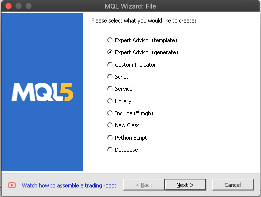
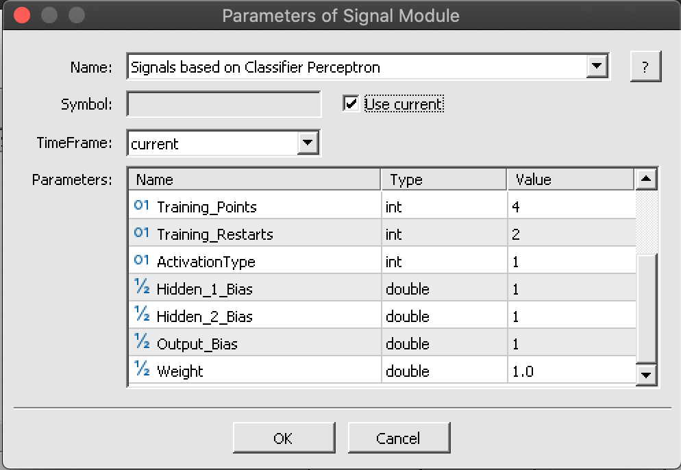
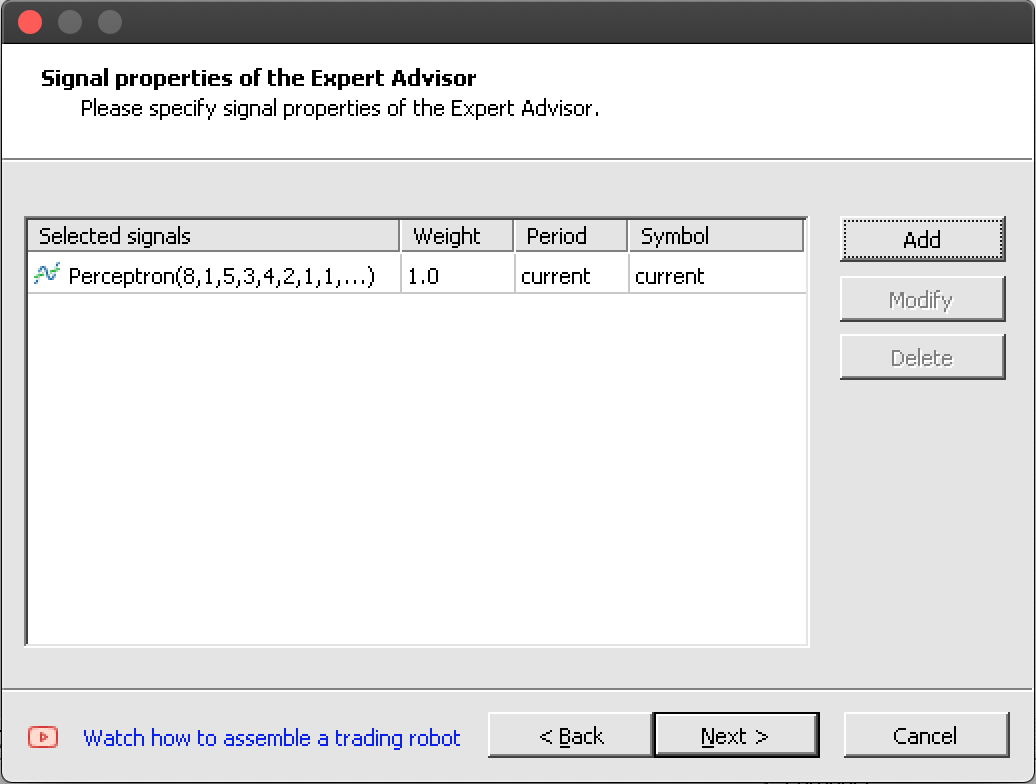
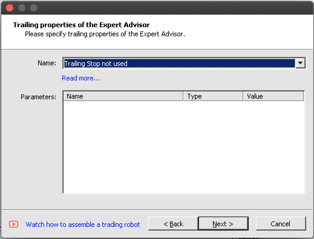
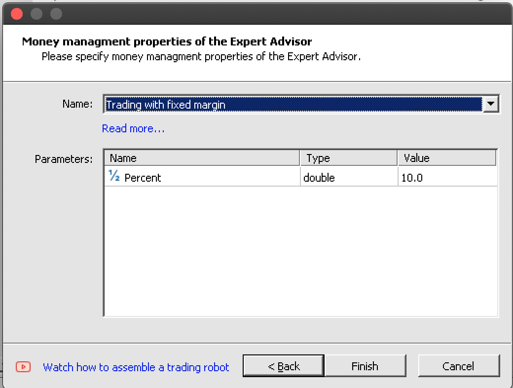
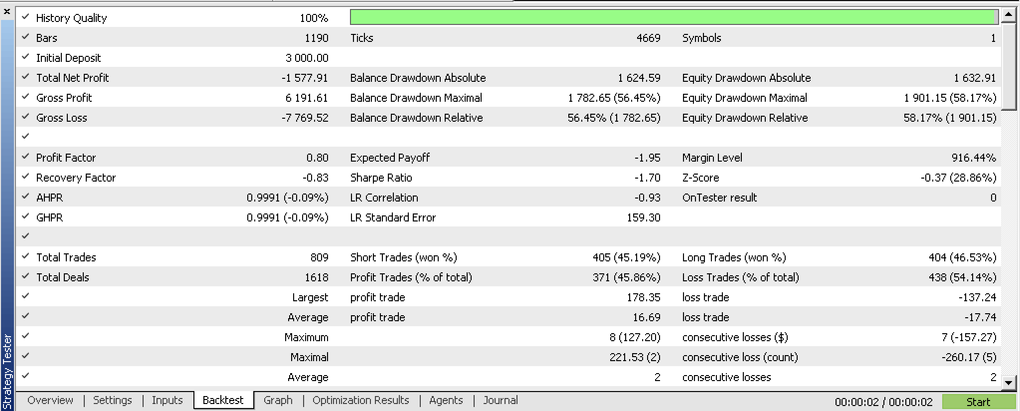
If we run a back test on our compiled expert before any optimization we get the following report:

If we perform optimizations of our expert adviser with a walk forward widow and get the following results:

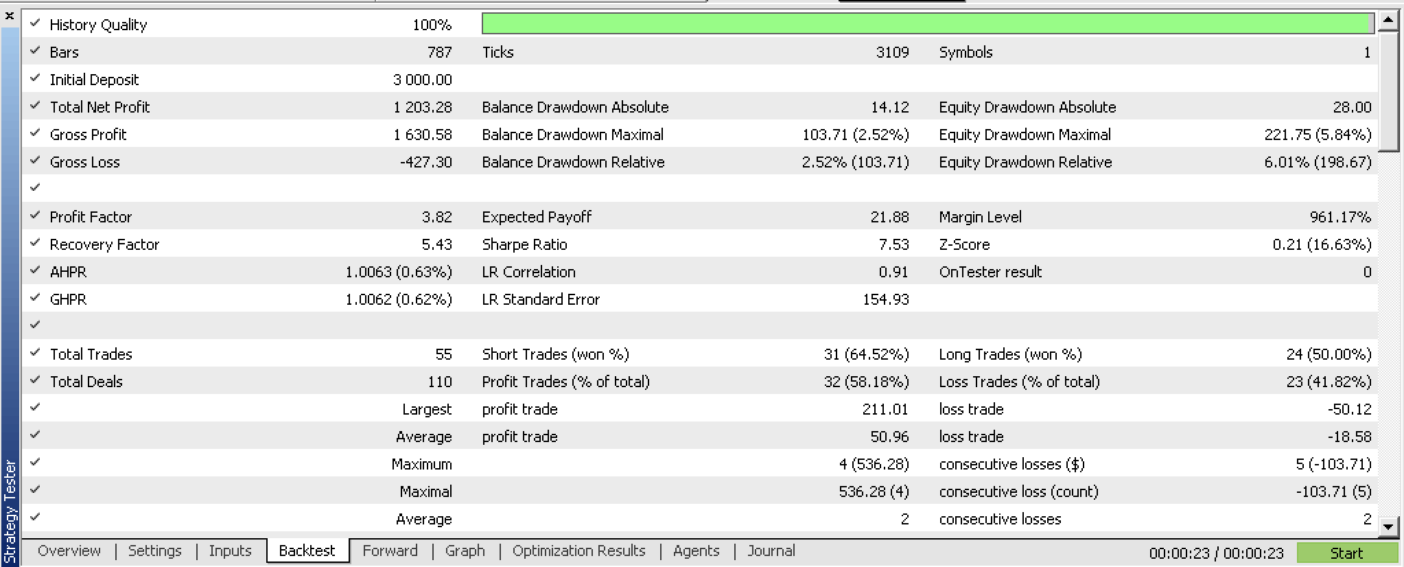
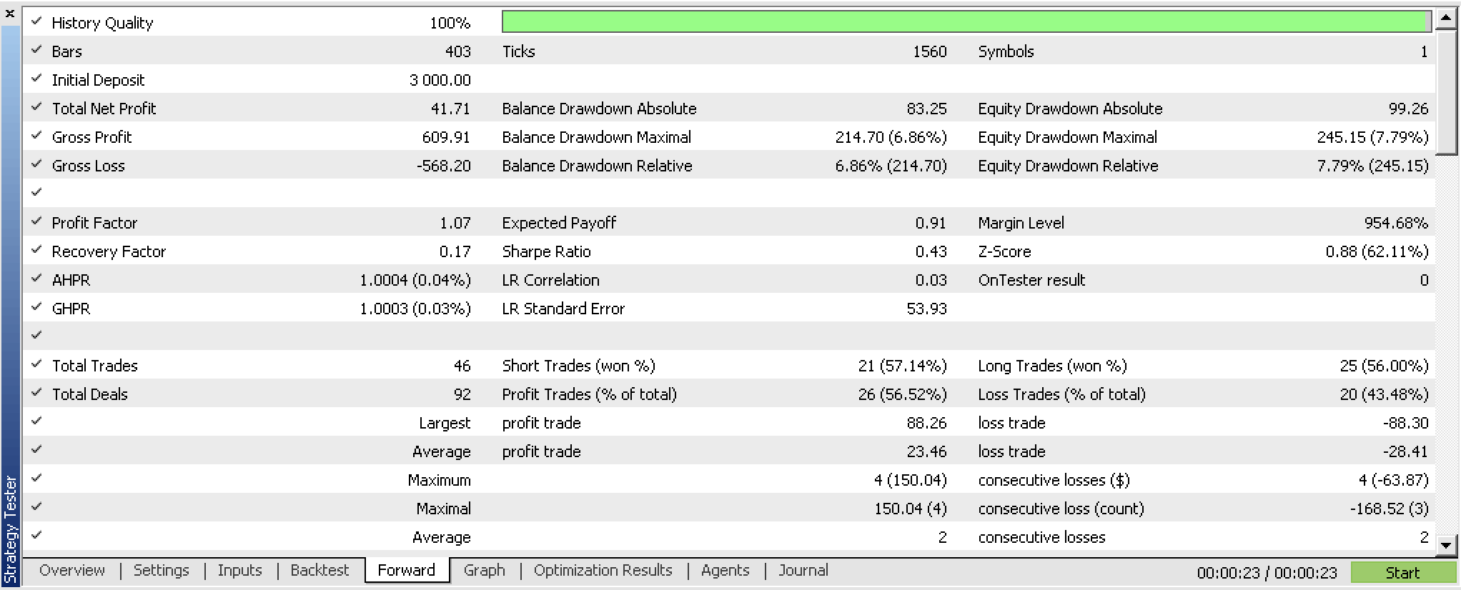
We have trained our perceptron and exported its weights based on optimization criteria of our expert adviser. A more succinct way to go about this would be to use inbuilt cross validation capabilities or even using something simpler like the root mean square error value of the report if bagging is not used. In either scenario we get to store weights that are more likely to match the training classifiers. From our tests the network is showing promise but as always more dilligence in testing over longer spans with your broker's tick data among other considerations, should be kept in mind.

Conclusion

To summarize, we have looked at how perceptrons can be implemented with minimal code on the part of the user thanks to Alglib code classes. We have highlighted a few preliminary steps, like data set normalization, that need to be taken before perceptrons are worth testing and learning from. In addition, we have shown extra measures that are worth considering once you have perceptrons that are ready to test. All these steps and extra measures, like the exporting of tunable parameters, are undertaken by ancillary code from the Alglib classes.

So, the advantages of using Alglib classes are primarily to minimize amount of code and the time it takes to have a testable system. But there are drawbacks none the less particularly when it comes to customization. For instance, our perceptrons cannot have more than 2 hidden layers. In scenarios where, complex data sets are being modelled this would be a bottleneck.