Discrete Hartley transform

Introduction

In 1942, Ralph Hartley proposed an analogue of the Fourier transform in his article "A More Symmetrical Fourier Analysis Applied to Transmission Problems".

Just like Fourier transform (FT), Hartley transform (HT) turns the original signal into a sum of trigonometric functions. But there is one significant difference between them. FT converts real values to complex numbers, while HT provides only real results. Because of this difference, the Hartley transform did not become popular - scientists and technicians did not see any advantages in it and continued to use the usual Fourier transform. In 1983, Ronald Bracewell presented a discrete version of the Hartley transform.

A bit of theory

Discrete Hartley transform (DHT) can be used in the analysis and processing of discrete time series. It allows filtering signals, analyzing their spectrum and much more. The capabilities of DHT are no less than those of the discrete Fourier transform. However, unlike DFT, DHT uses only real numbers, which makes it more convenient for implementation in practice, and the results of its application are more visual.

Let us have N real numbers h[0] … h[N-1]. Using the discrete Hartley transform, we obtain N real numbers H[0]…H[N-1] from them.

This transformation allows us to transfer a signal from the time domain to the frequency domain. With its help, we can estimate how great the influence of a particular harmonic in the original signal is. H[0] number contains basic information about the signal. H[1]…H[N-1] numbers provide additional data. These numbers show how strong a particular harmonic is in the original signal. The index of these numbers shows how many cycles of this harmonic will fit in the original signal. In other words, the higher the index, the higher the harmonic frequency.

Inverse Hartley transform is used to move from the frequency domain to the time domain. Its equation looks like this.

In both equations, the cas (cos and sin) function represents the sum of trigonometric functions.

Although, it can be replaced with a difference. The essence of the transformation will not change. Now, let's see how we can put DHT into practice.

Introducing discrete Hartley transform

So, DHT converts a signal from the time domain to the frequency domain. But is it possible to get any practical benefit from this?

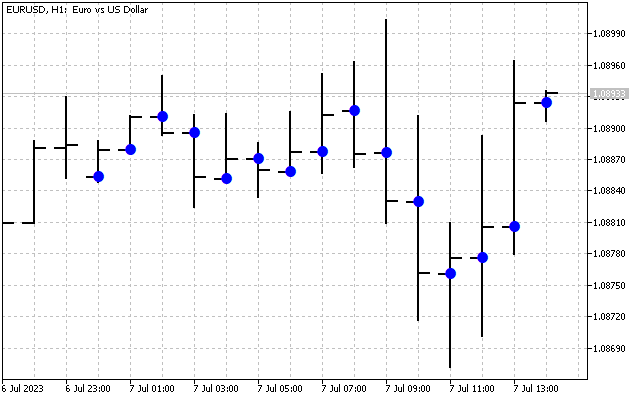
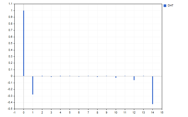
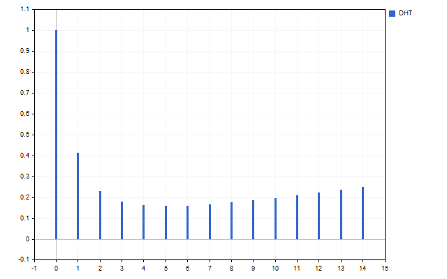
Let's take 15 Open prices as a signal. This is how the spectrum of this time series looks like (H[0] is not displayed due to scale differences).

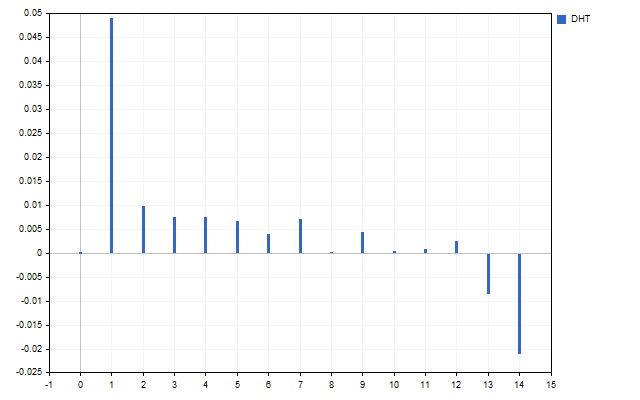
The figure clearly shows that different harmonics have different strengths. But what can be done with this spectrum?

Let's take simple moving average as an example. Its equation is very simple.

What will happen to the indicator if we set one of the prices to zero? It is unlikely we will get anything good. But in the frequency domain this is possible. We can zero out any number of harmonics.

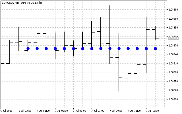
This is what the original signal looks like.

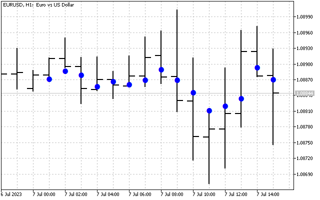
Now let's set all H[1] – H[14] harmonics to zero. Now we only have basic information about the original signal. Let's apply the inverse Hartley transform to this spectrum.

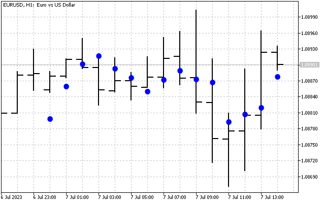
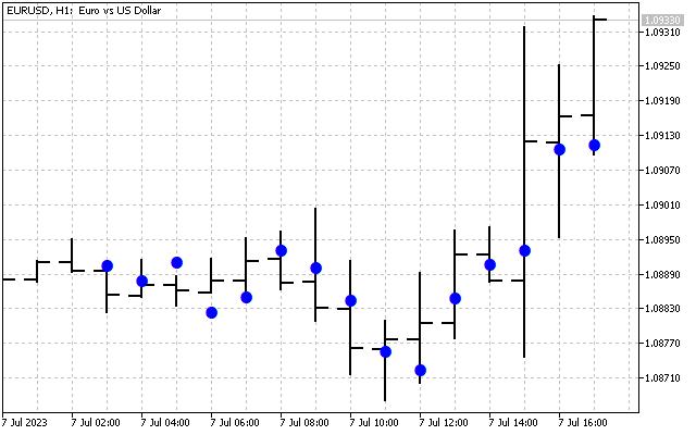
Now remove the harmonics with the highest frequencies H[10] – H[14]. The Hartley transform will provide the following result.

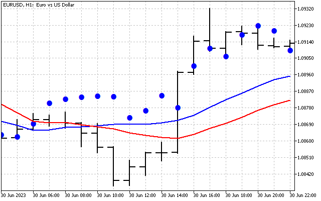
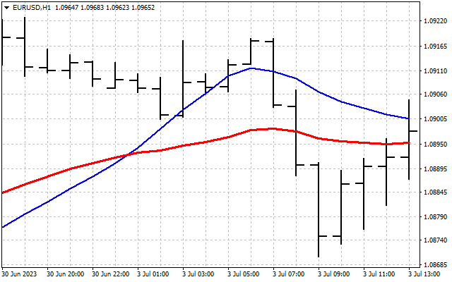
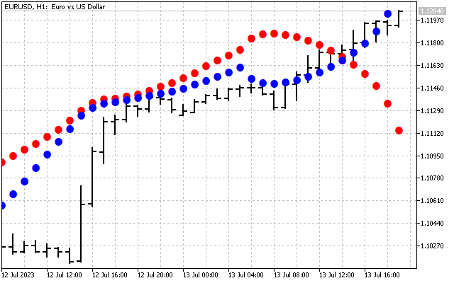
We have smoothed the original signal. Here is the first way to apply the Hartley transform in practice. First, we can smooth the time series in the frequency domain. After that, the obtained values are transferred to the input of the usual indicators. Let's take two moving averages as an example. One of them is applied to the price as usual (red line). The second one is applied to DHT values (blue line).

Nullifying some harmonics is not the only way to handle the signal spectrum. We can attenuate all harmonics at once, for example by dividing them by a given number.

Alternatively, we can attenuate each harmonic according to its frequency - the higher the frequency, the greater the attenuation.

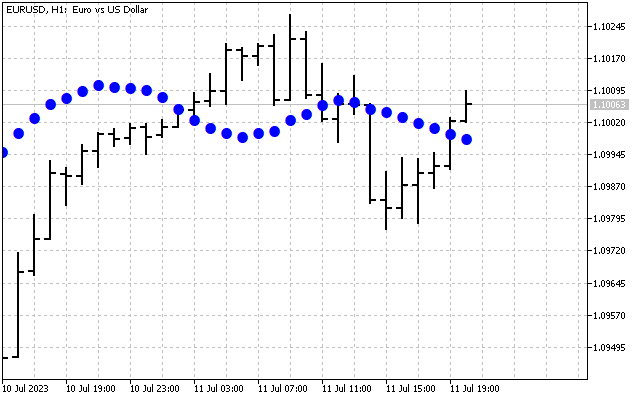
In any case, we will get a smoothed time series. This is what a signal looks like with harmonics attenuated by 2 times.

Another way to handle the spectrum is to leave only the strongest harmonics. To do this, we will have to find the average of all harmonics.

We will leave only those of them that exceed this average by their absolute value.

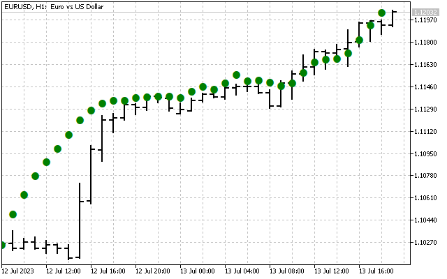
Then we will only have the main signal plus the strongest harmonics.

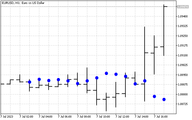
Another signal processing option is that we can reverse the harmonic values. Then the reconstructed signal will be in the opposite phase.

In this case, we will receive a mirror reflection of the signal - the upward trend is replaced by a downward one and vice versa. This approach can be useful when calculating support and resistance levels.

All options for processing the spectrum of the source signal can be used either individually or in combination with each other. For example, you can first leave only the strongest harmonics, and then change their sign to the opposite. In this case, the result will show a possible countertrend impulse.

Indicator with optimal spectrum

Any linear indicator is a set of coefficients. If we apply the Hartley transform to these coefficients, we obtain the spectral characteristic of the indicator.

We know thatSMA is a low pass filter. Let's check this statement. All coefficients of this indicator are equal to 1/N. The Hartley transform provides this indicator spectrum.

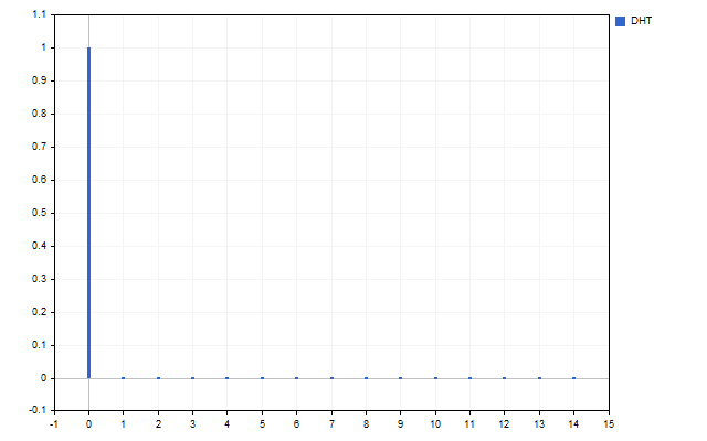
As we can see, SMA passes only the main signal H[0], but all other harmonics are completely suppressed.

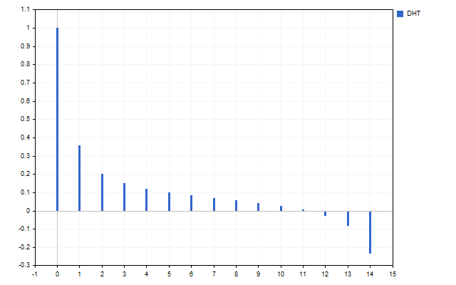
Spectra (frequency characteristics of indicators) can differ greatly from each other. For example, LWMA passes all harmonics of the input signal.

On the other hand, SMMA allows only some harmonics to pass through and suppresses the rest.

Each indicator has its own unique spectrum. It can be used to handle the price series. To do this, we need to first find the spectrum of the original signal H[]. Then we multiply it term by term by the spectrum of the indicator I[].

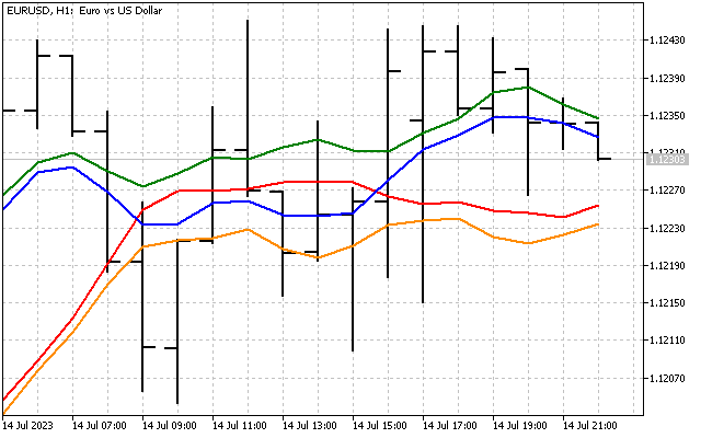
The inverse Hartley transform is applied to the obtained result. As a result, we obtain signal filtering in the frequency domain. This is what the operation of a frequency filter based on the LWMA indicator looks like.

But we can go the other way by first setting the spectrum of the indicator, and then getting its coefficients. Let's try to make an indicator whose spectral characteristic will correspond to the spectrum of the signal.

The algorithm will be as follows. First, we get the signal spectrum with DHT. Then we need to normalize it. To do this, we need to divide all harmonic values by D = H[0].

Note that after the normalization, H[0] = 1 is a mandatory condition when constructing an indicator.

After that, we need to apply the inverse transformation, which will provide the weighting coefficients of the indicator.

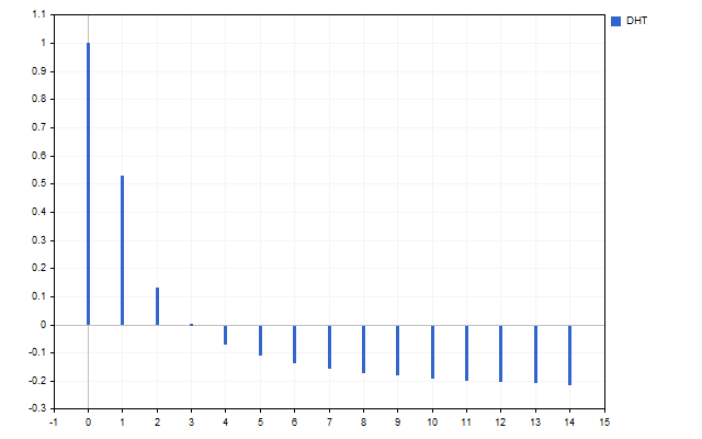
These coefficients are not very different from SMA. But such an indicator will have a smaller lag compared to the moving average, which will make it possible to more accurately track market dynamics.

Noise and color

When processing financial time series, the term "noise" most often refers to unwanted signal distortion. To eliminate such noise, a variety of filters can be used, including SMA.

A random or unpredictable signal can also be considered a noise. What happens if we represent market price movements as a sum of noises? To do this, we need to turn to the concept of colored noises. Colored noises are noises that have different energies in different frequency ranges. They got their name from the different colors of visible light: red is low-frequency noise, while violet is high-frequency noise.

Representing price movements as a sum of colored noises can give interesting results when analyzing financial time series. This approach allows us to take into account various frequency components of price movement.

Each colored noise has its own unique characteristic, which reflects the distribution of energy in the spectrum depending on the f frequency.

There are five primary colors of noise.

p parameter	noise color
-2	red
-1	pink
0	white
+1	blue
+2	violet

Each noise is associated with a specific price movement. For example, red noise can indicate the presence of long-term trends or cycles in price movements. White noise indicates that the market is in a flat state. Violet noise can indicate random and unpredictable price behavior. The use of colored noise in the analysis of financial time series can help to identify hidden patterns, as well as patterns that are not always visible in conventional analysis.

Now let's see how different noises behave in the market. To do this, we need to take a few simple steps.

First we need to find the spectrum of the signal, with which we can estimate the energy of each harmonic. To do this, we need to square the value of each harmonic.

Now, we can estimate the value of the scaling factor for noise with the p parameter. When using this coefficient, the total energies of the signal and noise will be equal.

Knowing this coefficient, we can construct the energy spectrum of EN[] noise.

Now we can find the HN[] noise spectrum. To do this, we need to take the square root of the energy spectrum.

There is very little left to do - assign +/- signs to the harmonics of the noise spectrum, just like the harmonics of the original signal. In this case, the noise and the original signal will be in the same phase.

After this, we need to perform an inverse Hartley transform to get the noise values on the price chart. This is what red noise looks like in the market.

But we can also take the opposite signs of the harmonics. In this case, the noise will be in the opposite phase with respect to the original signal. In addition, we can take strictly positive or negative harmonic values. We can afford this in the frequency domain. Then we will be able to see the boundaries of noise movements in the market.

The concept of colored noise can be used not only to describe market dynamics, but also to develop indicators.

To do this, we first need to set the indicator power E > 0. This parameter determines how sensitive the indicator will be. After this, we carry out the already familiar procedures. First we find the scaling factor.

After that, we find the spectrum of the HI[] indicator. Do not forget that HI[0] should be equal to 1.

All we have to do is assign +/- signs to the harmonics of the indicator spectrum if necessary. Then we need to apply the inverse Hartley transform and obtain the indicator coefficients. This is what a red noise indicator looks like with different variants of harmonic signs.

When developing indicators, we can use not only pure noise, but also their various combinations. For example, this is what the spectrum of the sum of red and violet noise looks like.

This is what the difference between the spectra of red and white noise looks like.

After receiving the coefficient[] indicator coefficients, we should normalize them. To do this, we first need to find the sum of all coefficients.

After this, we need to divide each coefficient by the resulting amount.

In addition to the main noises listed, there are others. For example, one definition of black noise is noise with the parameter p < -2. Let's try a different approach. Let us assume that the p noise parameter can take fractional values. Let's see how it changes over time.

To calculate the noise parameter, we first need to find the energy spectrum of the signal E[]. After this, we need to calculate four coefficients.

In all equations, k = 1…N-1. The most suitable noise parameter can be calculated using the equation.

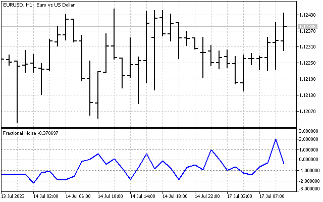
This is how this parameter changes in market conditions.

As we can see, the use of colored noise in financial time series analysis can be a useful tool for exploring and understanding market dynamics. This approach can help reveal hidden patterns and improve forecasting of price movements.

Conclusion

The discrete Hartley transform has its own fast transformation algorithms. But if we allocate the array for cas values beforehand, we can significantly speed up the data handling speed. The size of this array should be equal to (N-1)^2+1, where N is an indicator period. Then the values of this array are set as follows:

I used exactly this approach in this article.

The following indicators are attached to the article.

Symbol	Description
DHT	The indicator demonstrates the capabilities of processing signal harmonics. iPeriod - indicator period; CutOff - number of harmonics of the original signal to be left. If CutOff=0, then all harmonics remain; Constant - weakening a signal harmonics by a constant; Hyperbolic - suppression of harmonics according to the hyperbolic law; Strong - preservation of the original signal phase; Inverse - signal phase change;
DHT LWMA	The indicator shows price processing by the LWMA indicator in the spectral region
Spectrum	The indicator whose coefficients give a spectral characteristic similar to that of the original signal
Noise Levels	The indicator shows the levels of colored noises. Noise - noise color Type - change the phase of the original signal
Noise Indicator	The indicator selects coefficients corresponding to the selected noise color. E - noise power.
Fractional Noise	The indicator displaying the fractional noise parameter.