Pair trading

Introduction

Currently, there are a huge number of trading strategies for every taste. All these strategies are aimed at making a profit. But making a profit is in one way or another connected with the risks - the greater the expected profit, the higher the risks. A logical question arises: is it possible to reduce trading risks to a minimum, while receiving small but stable profits? These conditions are met by pair trading.

Pair trading is a variery of statistical arbitrage first proposed by Jerry Bamberger in the 1980s. This trading strategy is market neutral, allowing traders to profit in almost any market condition. Pair trading is based on the assumption that the characteristics of interrelated financial instruments will return to their historical averages after a temporary deviation. Thus, pair trading comes down to a few simple operations:

• identify discrepancies in the statistical relationship between two financial instruments;

• open positions on them;

• close positions when the characteristics of the instruments return to the average.

Despite its apparent simplicity, pair trading is not an easy or risk-free way to make a profit. The market is constantly changing and statistical relationships may change as well. Besides, any unlikely price movement could result in significant losses. Dealing with such adverse situations requires strict adherence to the trading strategy and risk management rules.

Correlation

Pair trading strategies are most often based on the correlation of two financial instruments. Changes in the prices of several currency pairs can be interrelated. For example, the price of one symbol moves in the same direction as the price of another symbol. In this case, there is a positive correlation between these symbols. In case of a negative correlation, prices move in opposite directions.

The correlation based pair trading strategy is very simple. First, traders should select two financial instruments with a strong correlation. Then they needs to analyze the change in correlation using historical data. Based on this analysis, traders can make an informed decision about entering a trade.

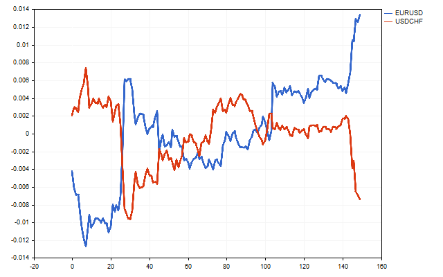
For trading, the most interesting currency pairs are those with negative correlation. For example, this is what the movement of EURUSD and USDCHF looks like.

Pearson correlation coefficient is the most commonly used method for estimating correlation. This coefficient is calculated by the equation:

This calculation always yields a biased estimate. In small samples, the resulting estimate of r may be very different from the exact correlation value. To reduce this error, we can use Olkin-Pratt adjustment:

Let's try to develop rules for a trading strategy based on correlation.

First, we need to select two suitable currency pairs. At the same time, the average correlation value of these pairs in history should be negative. Less is better.

Next, we need to collect statistics with sample correlation values on the history of these currency pairs. These statistics will be needed to calculate the signals.

The next step is to set the trigger level. If the current correlation reaches this level, the EA can open positions. This level can be set explicitly. For example, -0.95, -0.9 etc. There is also an alternative approach. We can take the historical correlation values and sort them in ascending order. As the response level, we can take the limit of 10% of the lowest values.

Before opening positions, we need to determine their type. If the current price of a currency pair is below the moving average, then a Buy position is opened for this symbol. Conversely, if the price is above the average, then a Sell position is opened. In this case, the positions opened should be multidirectional. This condition must be met, otherwise opening positions is prohibited.

In addition, the volumes of positions for different instruments should be interrelated. Suppose that PointValue is a price of one point in the deposit currency. Then the position volumes should be such that equality is satisfied.

In this case, the price movement by the same number of points will give approximately the same result for each of the instruments.

In addition, I added two more levels to the EA. Crossing the first level indicates the need to transfer positions to breakeven. Its value is 33%. Crossing the second level leads to the closure of all positions. The closing level is 67%, but not more than zero. Changing these levels can greatly affect the EA profitability.

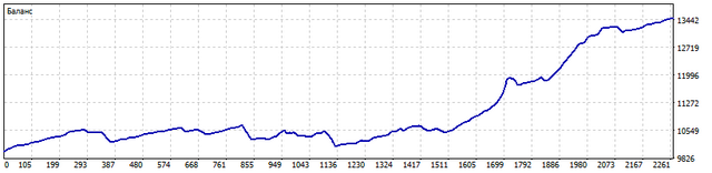
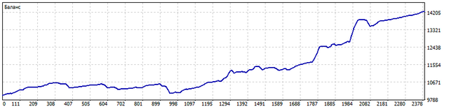
Let's test an EA following these rules. This is what the balance change looks like for EURUSD and USDCHF from 2021.01.01 to 2023.06.30.

Not bad. But the Pearson correlation coefficient has several features. Its use is justified only if the time series values have a normal distribution. Also, this coefficient is significantly influenced by spikes. Besides, Pearson correlation can only recognize linear relationships. To illustrate these features, it is best to use Anscombe's quartet.

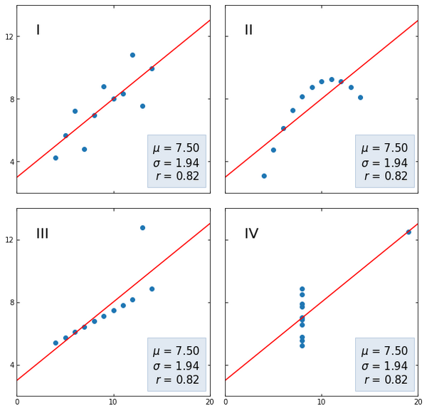
The first graph shows a linear correlation without any peculiarities. The second set of data features a nonlinear relationship, the strength of which the Pearson coefficient could not reveal. In the third set, the correlation coefficient is influenced by a strong spike. There is no correlation in the fourth graph, but nevertheless, even one value is enough for a fairly strong correlation to appear.

Spearman's rank correlation coefficient is free from these shortcomings. It captures the constantly increasing or decreasing dependence of two time series pretty well. For Spearman correlation, it does not matter according to which law the original data are distributed. The Pearson coefficient only works well with data that is normally distributed. Conversely, the Spearman coefficient can easily cope with any other distribution or their combination.

Also, the Spearman correlation coefficient can reveal nonlinear relationships. For example, one time series has a linear trend, while another has an exponential one. The Spearman coefficient can easily handle this situation, while the Pearson coefficient will not be able to fully reveal the strength of the relationship between these series.

We can calculate the Spearman rank correlation coefficient as follows. First we need to create two arrays. In each array, we will write the price value and bar index for both symbols.

index	EURUSD	USDCHF
0	1.06994	0.89312
1	1.06980	0.89342
2	1.07058	0.89277
3	1.07045	0.89294
4	1.07089	0.89283

Now we need to sort both arrays in ascending order. After sorting, the price values are of no interest to us. We only care about the index values that were before sorting and the current ones. The numbers in brackets are the price indices that were before the arrays sorting.

cur. index	EURUSD	USDCHF
0	1.06980   (1)	0.89277   (2)
1	1.06994   (0)	0.89283   (4)
2	1.07045  (3)	0.89294   (3)
3	1.07058   (2)	0.89312   (0)
4	1.07089   (4)	0.89342   (1)

Now we need to find the differences between the current indices of prices with the same indices before sorting. For example, let's find the difference D0. First, let's find the price index, which was equal to zero. These are 1.06994 EURUSD and 0.89312 USDCHF. The current indices of these prices are 1 and 3. Then, the difference D0 = 1 – 3 = -2.

Next, find the difference D1. The current price index of 1.06980 EURUSD is 0, and the price index of 0.89342 USDCHF is 4. D1 = 0 – 4 = -4.

The remaining differences are calculated in the same way.

After we have calculated all the differences, we can calculate the Spearman rank correlation coefficient:

At first glance, the difference between the Pearson and Spearman coefficients is small.

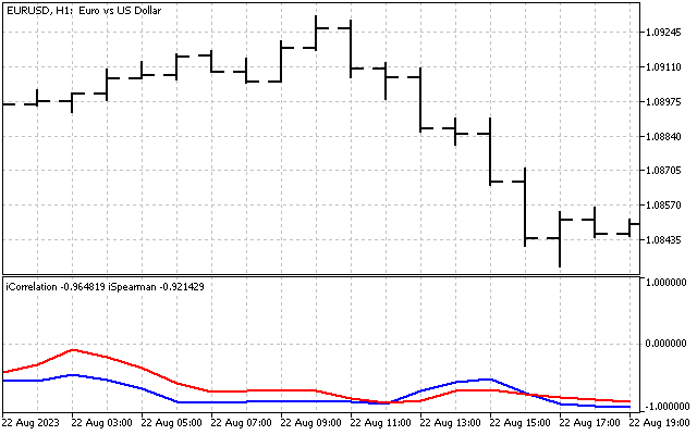
But it can have a significant impact on trading results. Testing the EA with the same parameters showed a better result compared to the Pearson coefficient.

It should be remembered that the trading strategy used can be significantly improved. For example, we can use a trailing stop instead of strictly transferring positions to breakeven, while the use of stop loss and take profit helps reducing the load on the deposit.

Much attention should be paid to the choice of the correlation period. The trading style depends on it. A short correlation period indicates a scalping nature of trading, and a large period indicates a trend-following one.

Cointegration

In 1980s, Clive Granger came up with the concept of time series cointegration. Since there is cointegration, then there should be integration first. Let's see what it is.

Let's assume that we have a time series whose values change according to the following law:

where c is a constant, while rand is a random number. The equation looks simple, but it can be used to create interesting motion trajectories. To generate random numbers, we will use the Statistics library. This library has all the necessary distributions allowing us to generate integrated time series.

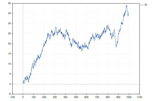
For example, this is what a movement looks like, in which the random component is subject to a uniform distribution.

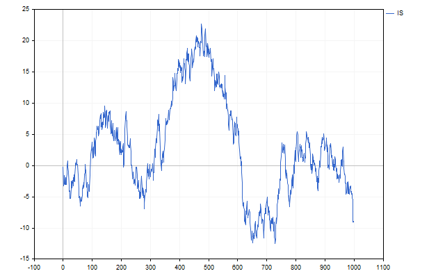
Does it look like a price chart? Now let's replace the uniform distribution with a normal one. We will get a chart more similar to the price movement.

But still something is missing. Price charts often feature gaps. Let's take the sum of the normal distribution and the Cauchy distribution as a random variable. It is this distribution that is responsible for black swans, white crows and other surprises. As a result, we get the following time series.

Is it possible to somehow use all this integration in trading? Let us assume that we have two integrated series, the random increments of which obey the same law, albeit with different parameters. If we find the difference between these series, then we can expect that the random components of both series will cancel each other out. Then we will be able to identify long-term relationships between these series, and the series themselves will be cointegrated.

In practice, the behavior of cointegrated currency pairs can be monitored using the difference:

k and m ratios should be selected in such a way that the d[i] values deviate from zero as little as possible. Their values can be estimated using the least squares method using the equations:

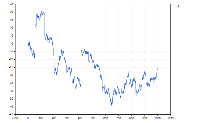
This is what the change in the difference between USDCHF and USDCAD looks like.

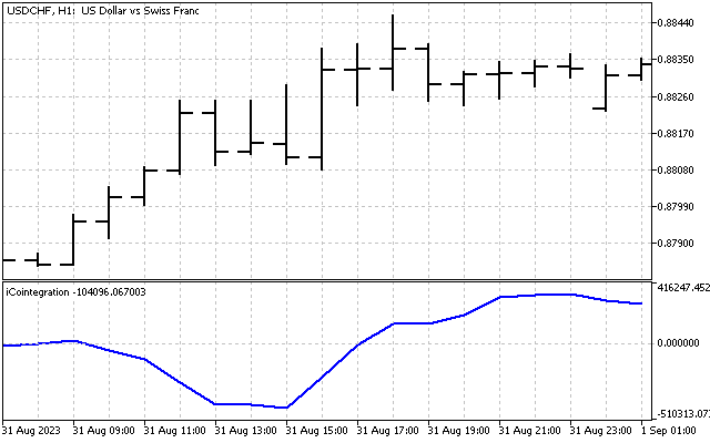
The value of this difference is not limited in any way either above or below. Its behavior in history is the main criterion when choosing cointegrated pairs. This difference should fluctuate around zero and change sign. The more such changes in signs in history, the better.

The trading strategy for cointegrated currency pairs is simple, and in many ways resembles the correlation strategy. The opening of two oppositely directed positions occurs when the difference between the two instruments reaches a certain maximum or minimum value. These positions must be closed when the difference becomes zero.

The EA working on USDCHF and USDCAD showed the following change in the trade balance for the period from 2021.01.01 to 2023.06.30.

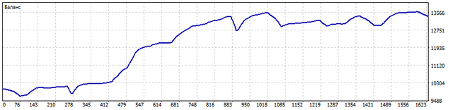
To improve the quality of EA trading, the same recommendations apply as for the correlation-based EA.

Conclusion

As you can see, pair trading strategies are quite usable. However, they require careful study and refinement for practical application.

The following programs were used when writing the article:

Name	Type	Features
sPearson	script	iPeriod - correlation period Analyzes historical correlations for all symbols available in Market Watch. Upon completion, saves the average correlation values in the Files folder
iPearson	indicator	SecSymbol - second symbol iPeriod - correlation period Shows the current Pearson correlation coefficient
sSpearman	script	Analyzes historical Spearman correlation
iSpearman	indicator	Shows the current Spearman correlation
EA Correlation	EA	EA based on Pearson and Spearman correlations
Integrated Series	script	The script shows the capabilities of constructing integrated time series. It is possible to use different distributions
sCointegration	script	The script evaluates possible cointegration of currency pairs
iCointegration	indicator	The indicator shows the cointegration difference between two currency pairs
EA Cointegration	EA	The EA applying cointegration of currency pairs for trading