

机器学习中的高斯过程(第二部分):在 MQL5 中实现和测试分类模型
 44
 4

引言
在上一篇文章中,我们学习了贝叶斯机器学习模型 — 高斯过程(Gaussian Processes)的理论基础,并开始在 MQL5 中创建一个 GP 库,描述了两个关键类:GaussianProcess 和 GPOptimizationObjective。
接下来,我们将详细介绍关键接口的实现,从而完善该库:IKernel、ILikelihood 和 IInference。之后,我们将使用合成数据测试该库,并编写分类和回归指标,以演示其在线模式下的运行 — 即在每根新 K 线上重新训练模型。
IKernel 接口
您可以在 Kernels.mqh 文件中找到的 IKernel 接口,是我们库中实现协方差核函数的基础。它使系统变得灵活且易于扩展:您可以在不改变代码主体结构的情况下,添加新的核函数类型或其组合。
interface IKernel { // Calculate the covariance matrix between two data sets virtual matrix Compute(const matrix &X1, const matrix &X2) = 0; // Calculate the derivative of the covariance matrix with respect to the given hyperparameter // param_index: index of the hyperparameter by which the derivative is taken (starting from 0) virtual matrix ComputeDerivative(int param_index) = 0; // Return the current values of all kernel hyperparameters virtual vector GetHyperparameters() const = 0; // Set new values for kernel hyperparameters virtual void SetHyperparameters(const vector ¶ms) = 0; // Return the number of kernel hyperparameters virtual int GetNumHyperparameters() const = 0; // Return the kernel string name virtual string GetName() const = 0; };
该接口定义了任何核函数操作所依赖的两个最重要的方法:
- Compute(const matrix &X1, const matrix &X2) — 计算两个数据集之间的 K 协方差矩阵。
- ComputeDerivative(int param_index) — 计算协方差矩阵对某个核超参数的导数。param_index 指定要计算导数的超参数索引。
RBFKernel 类(径向基核)
RBFKernel,也称为高斯核或平方指数核,是最常用的协方差核函数之一。它由两个超参数来表征:信号方差 σ_f(振幅)和长度尺度 l,长度尺度 l 决定了函数的平滑度。
//+------------------------------------------------------------------+ //| Kernel RBF class | //+------------------------------------------------------------------+ class RBFKernel : public IKernel { private: double length; double sigma_f; int n; // Number of rows in X1; int m; // Number of rows in X2; matrix m_K; matrix m_D_sq; // matrix of squared distances ||x_i - x_j||^2 public: //Constructor RBFKernel(double ls, double sf) : length(ls), sigma_f(sf) {} //Destructor ~RBFKernel() {} matrix Compute(const matrix &X1, const matrix &X2) override { n = (int)X1.Rows(); m = (int)X2.Rows(); matrix XX(n, m); if (!XX.GeMM(X1, X2.Transpose(), 1.0, 0.0)) { Print("Error: Failed to calculate XX = X * X^T"); return matrix::Zeros(n, m); } matrix diag1(n, 1); matrix X1_sq = X1 @ X1.Transpose(); diag1.Col(X1_sq.Diag(), 0); matrix diag2(m, 1); matrix X2_sq = X2 @ X2.Transpose(); diag2.Col(X2_sq.Diag(), 0); m_D_sq = matrix::Ones(n, 1) @ diag2.Transpose() + diag1 @ matrix::Ones(1, m) - 2 * XX; m_K = sigma_f * sigma_f * MathExp((-1 * m_D_sq) / (2 * length * length)); return m_K; } matrix ComputeDerivative(int param_index) override { matrix dK(n, m); switch (param_index) { case 0: { dK = (2.0 / sigma_f) * m_K; break; } case 1: { dK = m_K * (m_D_sq / (length * length * length)); break; } } return dK; } vector GetHyperparameters() const override { vector params(2); params[0] = sigma_f; params[1] = length; return params; } void SetHyperparameters(const vector ¶ms) override { if (params.Size() == 2) { sigma_f = params[0]; length = params[1]; } } int GetNumHyperparameters() const override { return 2; } string GetName() const override { return "RBFKernel"; } };
幸运的是,对于 RBF 核函数,很容易找到其导数:
-
对 sigma_f 的导数:

- 关于 l 的导数:

对于 “length” 参数,我们将 K 矩阵逐元素乘以 (D_sq / length^3),其中 D_sq 是平方欧氏距离矩阵。
LinearKernel 类(线性核)
LinearKernel 是一种简单的协方差核函数,它假设数据点之间存在线性关系。当预期函数可以用线性模型近似时,或者作为更复杂的复合核函数的组成部分时,通常会使用这种方法。
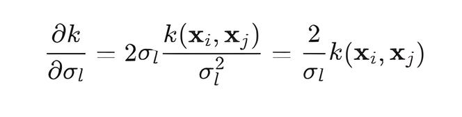
线性核函数有一个超参数:σ_l 信号方差。
//+------------------------------------------------------------------+ //| Linear kernel class | //+------------------------------------------------------------------+ class LinearKernel : public IKernel { private: double sigma_l; int n; int m; matrix m_K; public: //Constructor LinearKernel(double sl): sigma_l(sl){} //Destructor ~LinearKernel() {} matrix Compute(const matrix &X1, const matrix &X2) override { n = (int)X1.Rows(); m = (int)X2.Rows(); m_K.GeMM(X1, X2.Transpose(), sigma_l * sigma_l, 0.0); return m_K; } matrix ComputeDerivative(int param_index) override { matrix dK(n, m); switch (param_index) { case 0: { // Derivative with respect to sigma_l dK = (2.0 / sigma_l) * m_K; break; } } return dK; } vector GetHyperparameters() const override { vector params(1); params[0] = sigma_l; return params; } void SetHyperparameters(const vector ¶ms) override { if (params.Size() == 1) { sigma_l = params[0]; } } int GetNumHyperparameters() const override { return 1; } string GetName() const override { return "LinearKernel"; } };
ComputeDerivative(int param_index) 方法:
PeriodicKernel 类(周期核)
PeriodicKernel 用于对具有重复模式或季节性的数据进行建模,使其能够捕捉周期性依赖关系。
//+------------------------------------------------------------------+ //| Periodic kernel class | //+------------------------------------------------------------------+ class PeriodicKernel : public IKernel { private: double sigma_f; // Signal variance (oscillation amplitude) double length; // Scale length (smoothness of oscillations) double period; // Oscillation period int n; // Number of rows in X1 int m; // Number of rows in X2 matrix m_K; // Covariance matrix matrix m_D; // D matrix (sum of derivatives with respect to d [2 * sin^2(M_PI*distance/period] ) matrix m_distance_dim[]; // Array of difference matrices for each dimension |x_i_k - x_j_k| int m_d_cols; // Number of dimensions (features) (X.Cols()) public: //Constructor PeriodicKernel(double ls, double sf, double p) : sigma_f(sf), length(ls), period(p){} //Destructor ~PeriodicKernel() {} matrix Compute(const matrix &X1, const matrix &X2) override { n = (int)X1.Rows(); m = (int)X2.Rows(); int d = (int)X1.Cols(); m_d_cols = d; m_D = matrix::Zeros(n, m); ArrayResize(m_distance_dim, d); for (int k = 0; k < d; k++) { vector x1_k = X1.Col(k); vector x2_k = X2.Col(k); // Create a matrix where each column is a x1_k vector // (n x 1) * (1 x m) = (n x m) matrix x1_k_copy = x1_k.Outer(vector::Ones(m)) ; // Create a matrix where each row is the transposed vector of x2_k // (n x 1) * (1 x m) = (n x m) matrix x2_k_copy = vector::Ones(n).Outer(x2_k); // Calculate the matrix of all pairwise absolute differences between the elements of vectors x1_k and x2_k matrix distance = MathAbs(x1_k_copy - x2_k_copy); m_distance_dim[k] = distance; // Cache 'distance' for each dimension (feature) matrix sin_term = MathSin(M_PI * distance / period); sin_term = 2.0 * sin_term * sin_term; // 2 * sin^2(u) m_D += sin_term; // Sum up element by element } // Calculate the K matrix m_K = sigma_f * sigma_f * MathExp(-1 * m_D / (length * length)); return m_K; } matrix ComputeDerivative( int param_index) override { matrix dK(n, m); switch (param_index) { case 0: { // Derivative with respect to sigma_f // dK/d(sigma_f) = (2 / sigma_f) * K dK = (2.0 / sigma_f) * m_K; break; } case 1: { // Derivative with respect to 'length' // dK/d(length) = K * (2 * D / length^3) dK = m_K * ( 2.0 * m_D / (length * length * length) ); break; } case 2: { // Derivative with respect to 'period' // dK/d(period) = K * (-1/l^2) * dD/d(period) // dD/d(period) = Sum{k=1:d} (2 * pi * (x_ik - x_jk) / period^2) * sin(2*pi*(x_ik - x_jk)/period) matrix dD_dp = matrix::Zeros(n, m); for (int k = 0; k < m_d_cols; k++) { // Loop through each dimension (column) of the data matrix distance_k = m_distance_dim[k]; // matrix of absolute differences for the k-th dimension matrix u = M_PI * distance_k / period; // Calculate the argument u_k = pi * |x_ik - x_jk| / period matrix sin_2u = MathSin(2.0 * u); // Calculate sin(2 * u_k) // Use the already calculated u to calculate // -pi * |x_ik - x_jk| / period^2 matrix second_term = (-1*u) / period; // Accumulate dD/d(period) for the current measurement dD_dp += 2.0 * sin_2u * second_term; } // unite all parts of the derivative // dK = K * (-1/length^2) * dD_dp dK = m_K * (-1.0 / (length * length)) * dD_dp; break; } } return dK; } vector GetHyperparameters() const override { vector params(3); params[0] = sigma_f; params[1] = length; params[2] = period; return params; } void SetHyperparameters(const vector ¶ms) override { if (params.Size() == 3) { sigma_f = params[0]; length = params[1]; period = params[2]; } } int GetNumHyperparameters() const override { return 3; } string GetName() const override { return "PeriodicKernel"; } };
周期核函数关于 “period” 参数的导数:
计算关于周期参数的导数是最困难的,因为 “period” 位于三角函数内部,而三角函数又是指数函数的一部分。
导数公式基于链式法则,其中 K 取决于 D,而 D 通过正弦项取决于 “period”。ComputeDerivative 实现会迭代地计算每个维度的 dD_dp 分量,然后计算最终导数:
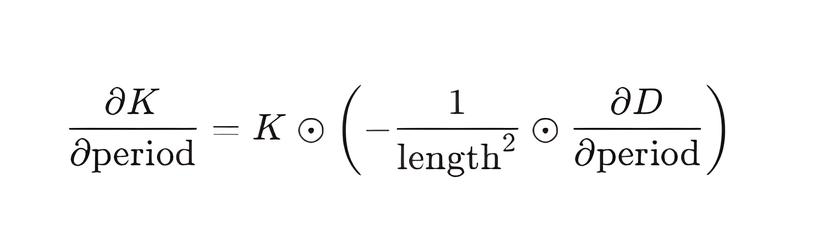
其中 dD_dp 计算为所有维度(特征)的导数 2 * sin^2(M_PI*distance/period)) 之和。
复合核函数
高斯过程允许将简单的协方差核函数进行组合,以创建能够描述数据不同方面(例如,趋势、周期性、噪声)的更复杂模型。此功能是通过两个复合核函数实现的:
- SumKernel — 通过求和多个核的协方差矩阵来组合这些核。
- ProductKernel — 通过按元素乘法计算多个核的协方差矩阵来组合这些核。
这两个类都管理其子核的超参数,将它们收集到一个共享向量中进行优化,然后再将其分发回去。
SumKernel 类
//+------------------------------------------------------------------+ //| Class for the sum of kernels | //+------------------------------------------------------------------+ class SumKernel : public IKernel { private: IKernel* kernels[]; public: // Constructor SumKernel(IKernel* &input_kernels[]) { ArrayResize(kernels, ArraySize(input_kernels)); ArrayCopy(kernels, input_kernels); } //Destructor ~SumKernel() { for (int i = 0; i < ArraySize(kernels); i++) { if (kernels[i] != NULL) { delete kernels[i]; } } ArrayFree(kernels); } matrix Compute(const matrix &X1, const matrix &X2) override { int n = (int)X1.Rows(); int m = (int)X2.Rows(); matrix sum = matrix::Zeros(n,m); for (int i = 0; i < ArraySize(kernels); i++) { sum += kernels[i].Compute(X1, X2); // Sum the matrices from each child kernel } return sum; } matrix ComputeDerivative(int param_index) override { int current_param_offset = 0; // Start at offset 0 for the first kernel for (int i = 0; i < ArraySize(kernels); i++) { // Get the number of hyperparameters of the current child kernel int num_params_current_kernel = kernels[i].GetNumHyperparameters(); // Check if the global param_index belongs to the current child kernel // param_index should be: // - greater than or equal to the current offset // - strictly less than the current offset + the number of parameters of the current kernel if (param_index >= current_param_offset && param_index < current_param_offset + num_params_current_kernel) { // If param_index belongs to this kernel, calculate its local index int local_param_index = param_index - current_param_offset; // Call ComputeDerivative on the found child kernel and // pass it the local index. // Since the derivative of the sum of kernels with respect to the parameter of one kernel is equal to the derivative // of this particular kernel by this parameter, we can immediately return the result return kernels[i].ComputeDerivative(local_param_index); } // If param_index does not belong to the current kernel, // increase the offset to check the next kernel current_param_offset += num_params_current_kernel; } Print("Error: SumKernel::ComputeDerivative - Parameter index ", param_index, " out of bounds"); return matrix::Zeros(1, 1); } //+---------------------------------------------------------------------------------+ //| The function returns the values of all hyperparameters of the composite kernel | //+---------------------------------------------------------------------------------+ vector GetHyperparameters() const override { vector all_params(GetNumHyperparameters()); int current_idx = 0; for (int i = 0; i < ArraySize(kernels); i++) { // Get the values of the parameters of the current child kernel vector kernel_params = kernels[i].GetHyperparameters(); for (int j = 0; j < (int)kernel_params.Size(); j++) { // Copy the parameters into the common vector all_params[current_idx + j] = kernel_params[j]; } // Update the offset for the next kernel current_idx += (int)kernel_params.Size(); } return all_params; } //+----------------------------------------------------------------------+ //|The function takes a vector of values of all hyperparameters, breaks | //|it into the appropriate parts and assigns them to each child kernel | //+----------------------------------------------------------------------+ void SetHyperparameters(const vector ¶ms) override { int current_idx = 0; for (int i = 0; i < ArraySize(kernels); i++) { // Get the number of hyperparameters of the current child kernel int num_params = kernels[i].GetNumHyperparameters(); vector sub_params(num_params); // Copy the corresponding parameters from the general vector for (int j = 0; j < num_params; j++) { sub_params[j] = params[current_idx + j]; } // Call the SetHyperparameters() method on the current child kernel, // passing it only its own parameters, collected in the sub_params vector kernels[i].SetHyperparameters(sub_params); current_idx += num_params; } } //+--------------------------------------------------------------------------------------+ //| Return the total number of hyperparameters for the entire SumKernel composite kernel | //+--------------------------------------------------------------------------------------+ int GetNumHyperparameters() const override { int total_params = 0; for (int i = 0; i < ArraySize(kernels); i++) { total_params += kernels[i].GetNumHyperparameters(); } return total_params; } string GetName() const override { string name = "Sum("; for (int i = 0; i < ArraySize(kernels); i++) { name += kernels[i].GetName(); if (i < ArraySize(kernels) - 1) name += ","; } name += ")"; return name; } //+------------------------------------------------------------------+ //| Provide external access to the list of child kernels | //+------------------------------------------------------------------+ void GetKernels(IKernel* &output_kernels[]) const { // Copy pointers from the internal kernels array to the passed // output_kernels external array. This provides access to child // kernels in the GaussianProcess::Fit() method, where it is necessary to iterate through // all elementary kernels to set optimization boundaries // of their hyperparameters. ArrayCopy(output_kernels, kernels); } };
- Compute 方法将最终的协方差矩阵 K 计算为每个子核返回的协方差矩阵的简单求和。这里运用了多态原理:尽管核数组存储的是 IKernel* 基类型的指针,但调用 kernels[i].Compute(X1, X2) 实际上会调用每个特定子核的特定 Compute 实现。这使得 SumKernel 可以与从 IKernel 继承的任何核函数一起使用。
- ComputeDerivative 方法的核心思想是,核函数之和的协方差函数关于特定超参数的导数,等于给定超参数所属的子核函数的协方差函数的导数。这意味着 ComputeDerivative 通过 param_index 找到对应的子核函数,并仅返回该核函数的导数。关于其他子核函数参数的导数被视为零。
ProductKernel 类
//+------------------------------------------------------------------+ //| Class for the product of kernels | //+------------------------------------------------------------------+ class ProductKernel : public IKernel { private: IKernel* kernels[]; matrix m_X1; matrix m_X2; int n; int m; public: // Constructor: copies pointers to child kernels ProductKernel(IKernel* &input_kernels[]) { ArrayResize(kernels, ArraySize(input_kernels)); ArrayCopy(kernels, input_kernels); } // Destructor ~ProductKernel() { for (int i = 0; i < ArraySize(kernels); i++) { if (kernels[i] != NULL){ delete kernels[i]; } } ArrayFree(kernels); } matrix Compute(const matrix &X1, const matrix &X2) override { n = (int)X1.Rows(); m = (int)X2.Rows(); m_X1 = X1; m_X2 = X2; matrix product = matrix:: Ones(n,m); for (int i = 0; i < ArraySize(kernels); i++) { // Polymorphism: call the Compute() method of each child kernel, // regardless of its specific type, and multiply the result element by element product *= kernels[i].Compute(X1, X2); } return product; } matrix ComputeDerivative(int param_index) override { matrix dK_prod(n, m); // Final derivative matrix int current_param_offset = 0; int target_kernel_idx = -1; // Kernel index the hyperparameter belongs to int local_param_index = -1; // Local index of the hyperparameter in this kernel // Step 1: Find the kernel and local index of the hyperparameter for (int i = 0; i < ArraySize(kernels); i++) { int num_params_current_kernel = kernels[i].GetNumHyperparameters(); if (param_index >= current_param_offset && param_index < current_param_offset + num_params_current_kernel) { target_kernel_idx = i; local_param_index = param_index - current_param_offset; break; } current_param_offset += num_params_current_kernel; } if (target_kernel_idx == -1) { Print("Error: ProductKernel::ComputeDerivative - Parameter index ", param_index, " out of bounds"); return matrix::Zeros(1, 1); } // Step 2: Calculate dK_k / d_theta_j for the target kernel matrix dK_target_kernel = kernels[target_kernel_idx].ComputeDerivative(local_param_index); // Step 3: Calculate the K_m product for all other kernels (m != k) matrix other_kernels_product = matrix::Ones(n, m); for (int i = 0; i < ArraySize(kernels); i++) { if (i != target_kernel_idx) { // Skip the target kernel other_kernels_product = other_kernels_product * kernels[i].Compute(m_X1, m_X2); } } // Step 4: Multiply the results element by element dK_prod = dK_target_kernel * other_kernels_product; return dK_prod; } // Collect the hyperparameter values of all child kernels into a single vector vector GetHyperparameters() const override { vector all_params(GetNumHyperparameters()); int current_idx = 0; for (int i = 0; i < ArraySize(kernels); i++) { vector kernel_params = kernels[i].GetHyperparameters(); for (int j = 0; j < (int)kernel_params.Size(); j++) { all_params[current_idx + j] = kernel_params[j]; } current_idx += (int)kernel_params.Size(); } return all_params; } void SetHyperparameters(const vector ¶ms) override { int current_idx = 0; for (int i = 0; i < ArraySize(kernels); i++) { int num_params_kernel = kernels[i].GetNumHyperparameters(); vector sub_params(num_params_kernel); for (int j = 0; j < num_params_kernel; j++) { sub_params[j] = params[current_idx + j]; } kernels[i].SetHyperparameters(sub_params); current_idx += num_params_kernel; } } int GetNumHyperparameters() const override { int total_params = 0; for (int i = 0; i < ArraySize(kernels); i++) { total_params += kernels[i].GetNumHyperparameters(); } return total_params; } string GetName() const override { string name = "Prod("; for (int i = 0; i < ArraySize(kernels); i++) { name += kernels[i].GetName(); if (i < ArraySize(kernels) - 1) name += "*"; } name += ")"; return name; } //+------------------------------------------------------------------+ //| Provide external access to the list of child kernels | //+------------------------------------------------------------------+ void GetKernels(IKernel* &output_kernels[]) const { ArrayCopy(output_kernels, kernels); } };
- Compute 方法将每个子核返回的协方差矩阵按元素相乘,得到最终的 K 个协方差矩阵。与 SumKernel 一样,这里也使用了多态性来调用相应子核函数的 Compute 方法。
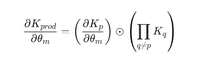
- ComputeDerivative 方法:为了计算 K 关于特定 K_p 子核的超参数的导数,ProductKernel 应用了乘积法则(莱布尼茨法则)。关于给定参数的导数等于 K_p 矩阵关于该参数的导数与所有其他子核的协方差矩阵的元素乘积(不考虑导数)的乘积:
ILikelihood 接口
ILikelihood 接口定义了我们库中的任何似然函数应该如何工作。它允许我们处理不同类型的数据,无论是连续值(如回归分析)还是离散类别(如分类分析)。
//+------------------------------------------------------------------+ //|Interface for likelihood functions | //+------------------------------------------------------------------+ interface ILikelihood { // Compute the p(y|f) log-likelihood for latent values f and observed values y virtual double LogLikelihood(const vector &f, const vector &y) = 0; //----------------------------- Derivatives of the logarithm of the likelihood with respect to f ----------------- // Calculate the vector of the first derivative of the log-likelihood with respect to f (dlp/df) virtual vector LogLikelihoodGradient(const vector &f, const vector &y) = 0; // Compute the second derivative (Hessian) matrix of the log-likelihood with respect to f (d^2lp/df df^T) virtual matrix LogLikelihoodHessian(const vector &f, const vector &y) = 0; // Calculate the vector of the third derivative of the log-likelihood with respect to f (d^3lp/df^3) virtual vector LogLikelihoodThirdDerivative(const vector &f, const vector &y) = 0; //----------------------------- Derivatives of the logarithm of the likelihood with respect to the parameters ----------------- // The first derivative of the log-likelihood with respect to the j-th likelihood hyperparameter. virtual double LogLikelihoodGradientParam(const vector &f, const vector &y, int param_index) = 0; // Hessian derivative of the log-likelihood with respect to the j-th likelihood hyperparameter. virtual matrix LogLikelihoodHessianDerivative(const vector &f, const vector &y, int param_index) = 0; // Return the name of the likelihood function virtual string GetName() const = 0; // Return the current values of the likelihood hyperparameters virtual vector GetHyperparameters() const = 0; // Set new values for the likelihood hyperparameters virtual void SetHyperparameters(const vector ¶ms) = 0; // Return the number of likelihood hyperparameters virtual int GetNumHyperparameters() const = 0; };
GaussianLikelihood 类
GaussianLikelihood 为回归问题实现了一个似然函数,该函数假设观测数据中的噪声服从正态分布。
//+------------------------------------------------------------------+ //| Gaussian likelihood class (for regression problems) | //+------------------------------------------------------------------+ class GaussianLikelihood : public ILikelihood { private: double m_noise_sigma; // Noise parameter (standard deviation) public: // Constructor GaussianLikelihood(double initial_noise_sigma) : m_noise_sigma(initial_noise_sigma) {} // Return the current value of the hyperparameter vector GetHyperparameters() const override { vector params(1); params[0] = m_noise_sigma; return params; } // Set a new hyperparameter value void SetHyperparameters(const vector ¶ms) override { if (params.Size() == 1) { m_noise_sigma = params[0]; } } // Return the number of hyperparameters int GetNumHyperparameters() const override { return 1; } // Calculate the log p(y|f) log-likelihood for a Gaussian distribution double LogLikelihood(const vector &f, const vector &y) override { int n = (int)y.Size(); double noise_variance = m_noise_sigma * m_noise_sigma; vector residual = y - f; // Formula for the logarithm of the density of a multivariate normal distribution return -0.5 / noise_variance * (residual @ residual) - 0.5 * n * MathLog(2 * M_PI * noise_variance); } //------------------ Derivatives with respect to f ----------------------- // Calculate the vector of the first derivative of the log-likelihood with respect to f (dlp/df) vector LogLikelihoodGradient(const vector &f, const vector &y) override { // d(log p(y|f))/df = (y - f) / sigma^2 return (y - f) / (m_noise_sigma * m_noise_sigma); } // Compute the second derivative (Hessian) matrix of the log-likelihood with respect to f (d^2lp/dfdf^T) matrix LogLikelihoodHessian(const vector &f, const vector &y) override { // d^2(log p(y|f))/dfdf^T = -1/sigma^2 * I int n = (int)y.Size(); return matrix::Identity(n, n) * (-1.0 / (m_noise_sigma * m_noise_sigma)); } // Calculate the vector of the third derivative of the log-likelihood with respect to f vector LogLikelihoodThirdDerivative(const vector &f, const vector &y) override { // For Gaussian likelihood d^3(log p(y|f))/df^3 = 0 return vector::Zeros((int)y.Size()); } // ------------------------------ Derivatives with respect to the parameter ----------------------------------- // // Calculate the first derivative of the log-likelihood with respect to the j-th likelihood hyperparameter virtual double LogLikelihoodGradientParam(const vector &f, const vector &y, int param_index) override { // Gaussian likelihood has only 1 hyperparameter: m_noise_sigma (index 0) if (param_index == 0) { // Formula for d(log p(y|f))/d(sigma_n): // = (y-f)^T(y-f) / sigma_n^3 - N / sigma_n vector y_minus_f = y - f; double sn3 = m_noise_sigma * m_noise_sigma * m_noise_sigma; double term1 = (y_minus_f @ y_minus_f) / sn3; double term2 = y.Size() / m_noise_sigma; // N / sigma_n return term1 - term2; } else { return 0.0; } } // Calculate the Hessian derivative of the log-likelihood with respect to the j-th likelihood hyperparameter matrix LogLikelihoodHessianDerivative(const vector &f, const vector &y, int param_index) override { int n = (int)y.Size(); if (param_index == 0) { // Derivative of Hessian with respect to m_noise_sigma: d/d(sigma_n) [-1/sigma_n^2 * I] = (2/sigma_n^3) * I double derivative_coeff = 2.0 / (m_noise_sigma * m_noise_sigma * m_noise_sigma); return matrix::Identity(n, n) * derivative_coeff; } else { return matrix::Zeros(n, n); } } string GetName() const override { return "GaussianLikelihood"; } };
主要方法:
- GaussianLikelihood 构造函数初始化一个超参数,即噪声标准差。
- LogLikelihood() — 计算多元正态分布概率密度函数的 p(y∣f) 对数似然值:

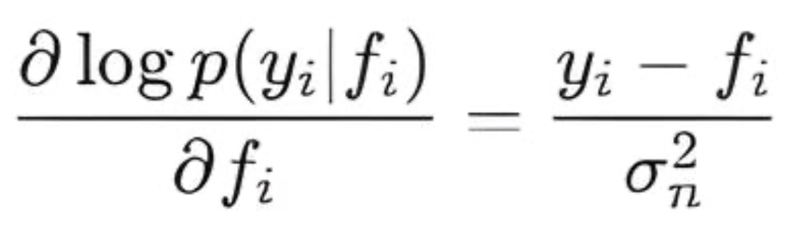
- LogLikelihoodGradient() — 计算对数似然关于函数f的潜在值的一阶导数。这是一个向量,其中每个元素都等于:
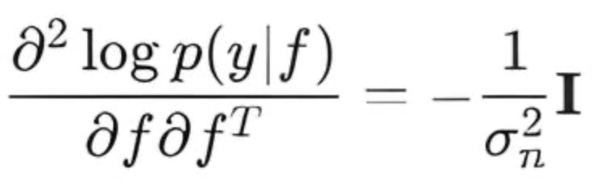
- LogLikelihoodHessian() — 计算对数似然函数关于 f 的二阶导数(Hessian)。对于高斯似然,Hessian是一个对角矩阵:
- LogLikelihoodThirdDerivative() — 计算三阶导数。对于高斯似然,所有高于二阶的导数均为零。
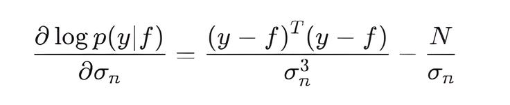
- LogLikelihoodGradientParam() — 计算对数似然函数关于超参数 m_noise_sigma 的一阶导数:
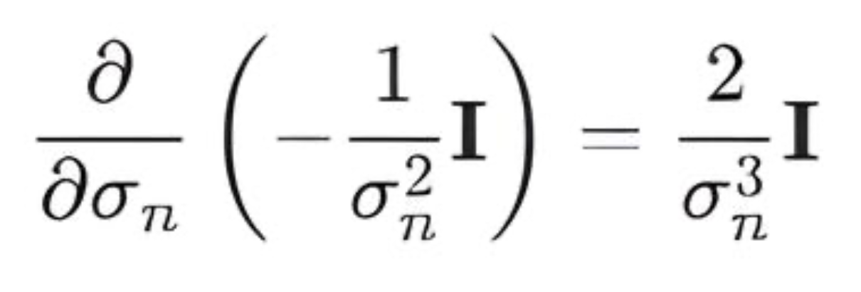
- LogLikelihoodHessianDerivative() — 计算对数似然函数关于超参数 m_noise_sigma 的 Hessian 导数:
LogitLikelihood 类
LogitLikelihood 用于二元分类,其中观测到的目标值 y 取值 {−1,+1}。它通过 sigmoid 函数将潜在函数 f 与类别成员概率联系起来。
LogitLikelihood 实现提供了 sigmoid() 和 Softplus() 辅助函数,这些函数会对输入值过大/过小的情况进行检查。
//+------------------------------------------------------------------+ //| Class for Logit likelihood (y {-1, +1}) | //+------------------------------------------------------------------+ class LogitLikelihood : public ILikelihood { public: // logit_sigmoid(x) = 1 / (1 + exp(-x)) double sigmoid(double x) const { if (x > 100.0) return 1.0; // Avoid NaN occurrences if (x < -100.0) return 0.0; return 1.0 / (1.0 + MathExp(-x)); } // Softplus log(1 + exp(x)) function double Softplus(double x) const { if (x > 100.0) return x; // For very large x, log(1 + exp(x)) ~ x if (x < -100.0) return MathExp(x); // For very small x, log(1 + exp(x)) ~ exp(x) return MathLog(1.0 + MathExp(x)); } public: // Constructor (logit likelihood has no hyperparameters of its own) LogitLikelihood() {} vector GetHyperparameters() const override { return vector::Zeros(0); } void SetHyperparameters(const vector ¶ms) override {} // Return the number of likelihood hyperparameters int GetNumHyperparameters() const override { return 0; } // --- Calculate the log-likelihood: log p(y|f) --- // Formula: sum_i (-log(1 + exp(-y_i * f_i))) double LogLikelihood(const vector &f, const vector &y) override { int n = (int)y.Size(); double total_log_likelihood = 0.0; for (int i = 0; i < n; i++) { total_log_likelihood += -Softplus(-y[i] * f[i]); } return total_log_likelihood; } // Compute the gradient of the log-likelihood with respect to f // Formula: d(log p(y_i|f_i))/df_i = y_i * sigma(-y_i * f_i) vector LogLikelihoodGradient(const vector &f, const vector &y) override { int n = (int)y.Size(); vector grad(n); for (int i = 0; i < n; i++) { grad[i] = y[i] * sigmoid(-y[i] * f[i]); // grad[i] = y[i] * (1 - sigmoid(y[i] * f[i])); equivalent to } return grad; } // Compute the Hessian of the log-likelihood of f (the H diagonal matrix) // Formula: d^2(log p(y_i|f_i))/df_i^2 = -sigma(y_i*f_i)(1 - sigma(y_i*f_i)) matrix LogLikelihoodHessian(const vector &f, const vector &y) override { int n = (int)y.Size(); matrix H = matrix::Identity(n, n); for (int i = 0; i < n; i++) { double sig = sigmoid(y[i] * f[i]); H[i][i] = -1*sig * (1.0 - sig); } return H; } // Calculate the third derivative of the log-likelihood with respect to f // Formula: d^3(log p(y_i|f_i))/df_i^3 = y_i * sigma(-y_i f_i) * (1 - sigma(-y_i f_i)) * (1 - 2*sigma(-y_i f_i)) vector LogLikelihoodThirdDerivative(const vector &f, const vector &y) override { int n = (int)y.Size(); vector third_deriv(n); for (int i = 0; i < n; i++) { double sig_neg_yf = sigmoid(-y[i] * f[i]); third_deriv[i] = y[i] * sig_neg_yf * (1.0 - sig_neg_yf) * (1.0 - 2.0 * sig_neg_yf); // equivalent to // double sig_yf = sigmoid(y[i] * f[i]); // third_deriv[i] = -y[i] * sig_yf * (1.0 - sig_yf) * (1.0 - 2.0 * sig_yf); } return third_deriv; } // LogitLikelihood has no hyperparameters virtual double LogLikelihoodGradientParam(const vector &f, const vector &y, int param_index) override { return 0.0; } // LogitLikelihood has no hyperparameters matrix LogLikelihoodHessianDerivative(const vector &f_latent, const vector &y, int param_index) override { int n = (int)y.Size(); return matrix::Zeros(n, n); } string GetName() const override { return "LogitLikelihood"; } };
主要方法:
- LogLikelihood() — 计算对数似然 logp(y∣f)。对于具有 y{-1,+1} 的二分类问题,这是二元交叉熵似然的对数之和:

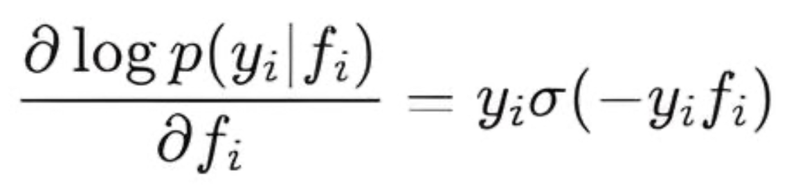
- LogLikelihoodGradient() — 计算对数似然函数对 f 的一阶导数。梯度向量的每个元素等于:
- LogLikelihoodHessian() — 计算对数似然函数关于 f 的二阶导数(Hessian 矩阵)。对于 LogitLikelihood,Hessian 矩阵是一个对角矩阵,其对角元素等于:
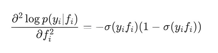
- LogLikelihoodThirdDerivative() — 计算对数似然函数关于 f 的三阶导数。向量中的每个元素都等于:

辅助函数和结构
StructUtils.mqh 文件包含一组枚举、数据结构和函数,使使用 GP 更加容易。
    enum PredictMode {
    PROBIT      = 0,  // Probit Approximation
    NUM_INTEGR  = 1,  // Numerical integration
    MONTE_CARLO = 2   // Monte Carlo

};

//--- Structure for prediction results
struct GPPredictionResult
{
    vector mu_f_star;    // Posterior mean for the latent f* function on new data
    matrix Sigma_f_star; // Posterior covariance for the latent f* function on new data

    // Regression-only fields (GaussianLikelihood)
    vector mu_y_star;      // Posterior mean of observations y*
    matrix Sigma_y_star;   // Posterior covariance of observations y*

    // Fields for classification only (LogitLikelihood, ProbitLikelihood, etc.)
    vector predicted_probabilities; // Probabilities p(y*=+1 | X*, D)
    vector predicted_labels;        // Predicted y* labels (+1 or -1)
};

// Structure for the inference result
struct GPInferenceResult {
    double      nlml_value;    // Negative logarithm of the marginal likelihood
    vector      nlml_gradient; // NLML gradient by kernel and likelihood hyperparameters

    // Inference results on training data:
    vector      mu_f_train;    // Posterior mean of the latent function f on the training data
    matrix      Sigma_f_train; // Posterior covariance of the latent function f on the training data (K^−1+W)^−1
    matrix      L_K_noisy;     // Cholesky decomposition K_noisy = cholesky(K + s2n*I)
    matrix      L_B;           // Cholesky decomposition B = I + W^0.5 @ K @ W^0.5
    matrix      sW;            // sW = W^0.5;
    vector      sW_diag;       // sW diagonal
    matrix      sW_K;          // sW @ K
    vector      alpha;         // (K_noisy)^-1 * y
    matrix      H;             // Hessian of the log likelihood d^2 log p(y|f)/df^2 (for LaplaceInference)
    bool        success;       // Flag indicating success of the inference function
};
- PredictMode 枚举定义了分类模型中执行预测的不同模式。
- GPInferenceResult 结构用于存储推理过程中获得的所有关键结果。
- GPPredictionResult 结构旨在存储对新(test)数据(X_test)执行预测后获得的所有结果。
- DiagonalTrace
//+-------------------------------------------------------------------+
//| Compute the trace of the product of two matrices using only       |
//| diagonal elements of the final matrix                             |
//+-------------------------------------------------------------------+
double DiagonalTrace(const matrix &A, const matrix &B)
  {
   ulong m = A.Rows();
   ulong n = A.Cols();
   ulong n_b = B.Rows();
   ulong p = B.Cols();
// Find the minimum size for the diagonal
   ulong k = MathMin(m, p);
   double tr = 0.0;

   for(ulong i = 0; i < k; i++)
     {
      // Dot product of the i-th row of A and the i-th column of B
      tr += A.Row(i)@B.Col(i);
     }
   return tr;
  }
计算两个矩阵 A 和 B 的乘积的迹 (Tr(A @ B)),而无需形成整个乘积矩阵。它通过将矩阵 A 的行和矩阵 B 的相应列的标量积相加来实现这一点。与全矩阵乘法相比,这可以显著降低计算成本。
- cho_solve (OpenBLAS LinearEquationsSolutionTriangular wrapper)
 //+-----------------------------------------------------------------------+
   //| Solve the system A*X = B using the Cholesky decomposition A = LL^T  |
   //| Parameters:                                                         |
   //|   c: Lower triangular matrix L from the Cholesky decomposition      |
   //|   b: right side of the system (matrix)                              |
   //| Return: matrix X - system solution                                  |
   //+---------------------------------------------------------------------+
   matrix            cho_solve(const matrix &c, const matrix &b)
     {
    // Check if 'c' matrix is lower triangular one
    if (!c.IsLowerTriangular()) {
        Print("Error: cho_solve - Input matrix 'c' is not lower triangular.");
        return matrix::Zeros(c.Rows(), b.Cols());
    }

// Step 1: Solve L * Y = B
    //  Y -  intermediate matrix, the result of solving L^-1 * B
    matrix Y;
    if (!c.LinearEquationsSolutionTriangular(EQUATIONSFORM_N, b, Y)) {
        PrintFormat("Error: cho_solve- LinearEquationsSolutionTriangular L * Y = B failed. Error Code: %d", GetLastError());
        return matrix::Zeros(c.Rows(), b.Cols());
    }

// Step 2: Solve L^T * X = Y
    //  X - L^T * X = Y system solution, which is equivalent to (L^T)^-1 * Y
    matrix X;
    if (!c.LinearEquationsSolutionTriangular(EQUATIONSFORM_T, Y, X)) {
        PrintFormat("Error: cho_solve- LinearEquationsSolutionTriangular L^T * X = Y failed. Error Code: %d", GetLastError());
        return matrix::Zeros(c.Rows(), b.Cols());
        }
      return X;
     }

   //+------------------------------------------------------------------+
   //| Solve the system Ax = b using the Cholesky decomposition A = LL^T|
   //| Parameters:                                                      |
   //|   c: Lower triangular matrix L from the Cholesky decomposition   |
   //|   b: right side of the system (vector)                           |
   //| Return: vector x - system solution                               |
   //+------------------------------------------------------------------+
   vector            cho_solve(const matrix &c, const vector &b)
     {
      // Check if 'c' matrix is lower triangular one
    if (!c.IsLowerTriangular()) {
        Print("Error: cho_solve - Input matrix 'c' is not lower triangular");
        return vector::Zeros(c.Rows());
    }

    // Step 1: Solve L * y = b
    // y - intermediate vector, the result of solving L^-1 * b
    vector y;
    if (!c.LinearEquationsSolutionTriangular(EQUATIONSFORM_N, b, y)) {
        PrintFormat("Error: cho_solve- LinearEquationsSolutionTriangular L * y = b failed. Error Code: %d", GetLastError());
        return vector::Zeros(c.Rows());
    }

    // Step 2: Solve L^T * x = y
    // x - final solution of the L^T * x = y system, which is equivalent to (L^T)^-1 * y
    vector x;
    if (!c.LinearEquationsSolutionTriangular(EQUATIONSFORM_T, y, x)) {
        PrintFormat("Error: cho_solve- LinearEquationsSolutionTriangular L^T * x = y failed. Error Code: %d", GetLastError());
        return vector::Zeros(c.Rows());
    }
      return x;
     }
cho_solve 函数旨在高效地求解线性方程组 Ax=b(或矩阵 B 的 AX=B),其中矩阵 A 由其 Cholesky 分解 A=LL^T 得到。这里 L 是一个下三角矩阵。
直接计算 A^−1 (A.Inv()) 需要消耗大量资源,并且数值可能不稳定。另一方面,Cholesky 分解提供了一种更高效、更稳健的方法。
cho_solve 函数内部执行两个主要操作:
- 前向代入:求解方程组 LY=B(或 Ly=b),其中 L 为输入矩阵 c,Y(或 y)为中间结果。由于 L 是三角矩阵,因此该解法相对较快。
- 反向代入:随后求解系统 L^TX=Y(或 L^Tx=y),其中 L^T 为矩阵 L 的转置。该方法同样高效,因为 L^T 是上三角矩阵。
这些运算是使用 OpenBLAS 高性能线性代数库中的 LinearEquationsSolutionTriangular 函数实现的。这提供了显著的计算速度,使其对于高斯过程等资源密集型机器学习模型来说是不可或缺的。
IInference 接口
interface IInference
  {
// This method performs inference (i.e., computes the posterior distribution of f)
// and returns the components needed for NLML and prediction
   virtual void Infer(const matrix &X, const vector &y,
                      IKernel *kernel, ILikelihood *likelihood,GPInferenceResult &result) = 0;
   virtual string GetName() const = 0;
  };
该接口允许在不同的推断方法之间切换,例如高斯似然的精确推理和非高斯情况的近似方法,而无需改变高斯过程的核心逻辑。
Infer 方法是此接口的核心。它对潜函数 f 的后验分布进行推断,并返回后续计算(NLML 与预测)所需的分量。它接受以下参数:
- X — 训练特征矩阵
- y — 训练标签向量,
- kernel — 指向 Ikernel 对象的指针,
- likelihood — 指向 ILikelihood 对象的指针,
- result — 对 GPInferenceResult 结构的引用,用于存储所有推断结果,包括:
- 超参数优化所需的边际似然(NLML)的负对数,
- 所有核函数和似然函数超参数的 NLML 梯度向量,
- 辅助矩阵和向量:(L_K_noisy、L_B、sW、mu_f_train、Sigma_f_train、alpha)用于计算 NLML 梯度和随后对新数据的预测。
ExactInference 类
//+------------------------------------------------------------------+
//| ExactInference For Gaussian likelihood only                      |
//+------------------------------------------------------------------+
class ExactInference : public IInference
  {

public:
                     ExactInference() {}

   void              Infer(const matrix &X, const vector &y,
                           IKernel *kernel, ILikelihood *likelihood,GPInferenceResult &result) override
     {
      if(likelihood.GetName() != "GaussianLikelihood")
        {
         Print("ExactInference supports only GaussianLikelihood");
         result.nlml_value = DBL_MAX;
         return;
        }
      result.success = false;
      int n = (int)y.Size();

      //  Calculate K with current kernel parameters
      matrix K = kernel.Compute(X, X);

      //  Get the noise variance
      vector likelihood_params = likelihood.GetHyperparameters();
      double sigma = likelihood_params[0];
      double variance = sigma * sigma;

      double jitter = 1e-6;
      matrix K_noisy = K + matrix::Identity(n, n) * (variance + jitter);

      if(!K_noisy.Cholesky(result.L_K_noisy))
        {
         PrintFormat("Error: Cholesky decomposition failed. Error Code: %d",GetLastError());
         result.nlml_value = DBL_MAX;
         return;
        }
      //------------- Algorithm 2.1 GPML ---------------------------
      //Calculate alpha (K_noisy^-1 * y) - O(N^2)
      result.alpha = cho_solve(result.L_K_noisy, y);
      //+------------------------------------------------------------------+
      //| NLML = 0.5y^T(K+σ^2*I)^-1*y + 0.5*log|K+σ^2*I| +n/2*Log(2π)      |
      //+------------------------------------------------------------------+
      //+------------------------------------------------------------------+
      //| NLML = 0.5y^T*alpha         + 0.5*log|K+σ^2*I| +n/2*Log(2π)      |
      //+------------------------------------------------------------------+
      // --- Calculate the first term in the NLML equation:
      double data_term = 0.5 * (y @ result.alpha);
      // --- Calculate the second term: 1/2 * log|K + sigma^2*I| = sum(log(L_ii))
      double log_det = MathLog(result.L_K_noisy.Diag()).Sum();
      // --- Calculate the third term: n/2 * log(2π)
      double const_term = 0.5 * n * MathLog(2 * M_PI);
      //--- NLML
      result.nlml_value = data_term + log_det + const_term;

      // -------------------- NLML gradients calculations --------------------------------------
      result.nlml_gradient.Resize(kernel.GetNumHyperparameters() + likelihood.GetNumHyperparameters());
      int current_grad_idx = 0;
      // Calculate (K_noisy^-1)
      matrix K_noisy_inv = cho_solve(result.L_K_noisy, matrix::Identity(n, n));

      // 1. Gradients on kernel hyperparameters
      vector kernel_hyperparams = kernel.GetHyperparameters();
      // Calculate aatK_noisy_inv once before the loop - O(N^2)
      matrix aatK_noisy_inv = result.alpha.Outer(result.alpha) - K_noisy_inv;
      matrix dK_dtheta;
      for(int i = 0; i < (int)kernel_hyperparams.Size(); i++)
        {
         dK_dtheta = kernel.ComputeDerivative(i); // O(N^2)
         result.nlml_gradient[current_grad_idx] = -0.5 * DiagonalTrace(aatK_noisy_inv, dK_dtheta);
         current_grad_idx++;
        }
      // 2. Gradient over noise hyperparameter
      // dNLML/d(sigma^2) = 0.5 * (trace(K_noisy^-1) - alpha^T * alpha )
      double dNLML_d_sigma2n = 0.5 * (K_noisy_inv.Trace() - result.alpha @ result.alpha);
      result.nlml_gradient[current_grad_idx] = dNLML_d_sigma2n * (2.0 * sigma);
      result.success = true;
     }

   string            GetName() const override { return "ExactInference"; }
  };
ExactInference 类旨在执行高斯过程 (GP) 中的精确推断,并且仅适用于使用高斯似然的情况。该实现的主要重点是高效计算 NLML 及其解析梯度。与数值方法相比,直接使用方程计算的分析梯度提供了更高的精度,并显著加快了优化过程。
推理算法由以下几个关键步骤组成:
- Knoisy 协方差矩阵的形成:首先,为训练数据计算 K 核协方差矩阵。然后将噪声方差(variance = sigma*sigma)和一个小的正抖动值(1e-6)加到 K 的对角元素上。这形成了 Knoisy 矩阵;
- αlpha 向量的计算;
- 负对数边际似然 (NLML) 计算;
- 计算 NLML 梯度以进行优化。
要计算所需的梯度和 NLML 本身,需要逆协方差矩阵 (K+σ2*I)^−1 和向量 α=(K+σ2*I)^−1 * y。
cho_solve 函数有助于尽快计算这些变量。

LaplaceInference 类
LaplaceInference 实现了拉普拉斯近似,这是一种适用于 GP 中回归和分类问题的近似推断方法。
//+------------------------------------------------------------------+
//| LaplaceInference                                                 |
//+------------------------------------------------------------------+
class LaplaceInference : public IInference
  {
private:
   int               m_max_iterations;
   double            m_tolerance;

public:
                     LaplaceInference(int max_iter = 100, double tolerance = 1e-10) :
                     m_max_iterations(max_iter),
                     m_tolerance(tolerance) {}

   void              Infer(const matrix &X_train, const vector &y,
                           IKernel *kernel, ILikelihood *likelihood, GPInferenceResult &result) override
     {
      result.success = false;
      int n = (int)y.Size();

      //  Calculate K
      matrix K = kernel.Compute(X_train, X_train);
      double jitter = 1e-6;
      K = K + matrix::Identity(n, n) * jitter;

      vector f = (result.mu_f_train.Size() == n) ? result.mu_f_train : vector::Zeros(n);
      bool converged = false;
      matrix W(n, n);                  // W := -Hessian
      matrix L_B(n, n);                // L := cholesky(I + W^0.5*K*W^0.5), B = I + W^0.5*K*W^0.5
      vector b(n);                     // b := Wf + grad loglike p(y|f)
      vector a(n);                     // a := b - W^0.5*L^T\(L\(W^0.5*K*b))
      matrix sW = matrix::Zeros(n, n); // W^0.5
      vector sW_diag(n);               // sqrt(W) vector for storing diagonal elements
      double prev_lml_value = -DBL_MAX; // For the convergence criterion according to LML
      double current_lml_value = -DBL_MAX;
      int iter;
      // --- Step 1: Finding the f_hat mode using Newton's method (According to 3.1 GPML Algorithm) ---
      for(iter = 0; iter < m_max_iterations; iter++)
        {
         // 1. W := - Hessian (diagonal matrix)
         W = -1 * likelihood.LogLikelihoodHessian(f, y);
         // Calculate sW_diag_vector (root of W)
         sW_diag = MathSqrt(W.Diag());
         // 2. L_B := cholesky(I + W^0.5*K*W^0.5)
         // Calculate sW_K = sW * K
         result.sW_K.Resize(n, n);
         for(int i = 0; i < n; i++)
           {
            result.sW_K.Row(sW_diag[i] * K.Row(i),i); // K[i,:] * sW_diag_vector[i]
           }
         // Calculate B = I + sW_K * sW
         matrix temp_sWKsW(n, n);
         for(int j = 0; j < n; j++)
           {
            temp_sWKsW.Col(result.sW_K.Col(j)*sW_diag[j],j) ; // sW_K[:,j] * sW_diag_vector[j]
           }
         matrix B = matrix::Identity(n, n) + temp_sWKsW;
         if(!B.Cholesky(L_B))
           {
            PrintFormat("Error:Cholesky decomposition of B failed. Error Code: %d", GetLastError());
            result.nlml_value = DBL_MAX;
            return;
           }
         result.L_B = L_B; // Save for use in forecasts
         // 3. b := W*f + grad loglike p(y|f)
         b = W.Diag() * f + likelihood.LogLikelihoodGradient(f, y);
         // 4. a := b - W^0.5*L_B^T\(L_B\(W^0.5*K*b))
         a = b - sW_diag*cho_solve(L_B,result.sW_K @ b);
         // 5. f := K * a (new Newton step)
         f = K @ a;

         // --- Calculate the current NLML for the convergence criterion ---
         double log_likelihood_at_f = likelihood.LogLikelihood(f, y);
         double sum_log_diag_L_B = MathLog(L_B.Diag()).Sum();
         current_lml_value = -0.5 * a @ f + log_likelihood_at_f - sum_log_diag_L_B;
         result.nlml_value = -current_lml_value;

         // 6. Convergence check
         double lml_change = current_lml_value - prev_lml_value;
        // PrintFormat("Iter %d: LML = %g, delta LML = %g",iter, current_lml_value, lml_change);

         // Check convergence by LML
         if((lml_change < m_tolerance))
           {
           // PrintFormat("Converged at iter %d: LML = %g, delta LML = %g",iter, current_lml_value, lml_change);
            converged = true;
            break;
           }
         prev_lml_value = current_lml_value;
        }

      if(!converged)
        {
         PrintFormat("Warning: Newton algorithm didn't converge at iteration %d. Final LML: %g (delta: %g, tolerance: %g)",
                     iter, current_lml_value, (current_lml_value - prev_lml_value), m_tolerance);
        }

      //---Save to the GPInferenceResult structure
      result.mu_f_train = f; // Posterior mean of the latent function at training points
      result.H = likelihood.LogLikelihoodHessian(f, y); // Hessian at point f_hat

      // --- Calculating analytical gradients NLML Algorithm 5.1 GPML ---
      result.nlml_gradient.Resize(kernel.GetNumHyperparameters() + likelihood.GetNumHyperparameters());
      int current_grad_idx = 0;
      // ==============================================================================
      // 1. Gradients on KERNEL hyperparameters
      // ==============================================================================
      //   Calculate R := W^0.5*L_B^-T*(L_B^-1*W^0.5)
      result.sW.Diag(sW_diag);
      matrix R(n,n);
      matrix cs = cho_solve(L_B,result.sW);
      for(int i = 0; i < n; i++)
        {
         R.Row(sW_diag[i] * cs.Row(i),i);
        }
      //  Calculate C := L_B^-1 * W^0.5 * K
      // To do this, solve the linear equation: L_B * C = sW * K relative to C
      matrix C;
      if(!L_B.LinearEquationsSolutionTriangular(EQUATIONSFORM_N,result.sW_K, C))
        {
         PrintFormat("Error: LinearEquationsSolutionTriangular L_B * C = W^0.5 * K.Error Code: %d", GetLastError());
         result.nlml_value = DBL_MAX;
         return;
        }
      // Calculate A = Sigma_f_train = (K^−1+W)^−1 = K - C^T @ C
      // Sigma_f_train - posterior covariance matrix of the latent f function on the training data
      matrix CTC = C.Transpose() @ C;
      result.Sigma_f_train = K - CTC;

      //------------------- grad NLML = -(s1 + s2^T*s3)
      // Calculate s2 (first implicit part)
      // s2 := -0.5 * diag( diag(K) - diag(C^T*C) ) * ThirdDerivative loglike by f
      vector third_deriv = likelihood.LogLikelihoodThirdDerivative(f, y);
      //matrix diag;
      //diag.Diag(K.Diag() - CTC.Diag());
      //vector s2 = -0.5 * diag  @ third_deriv;
      vector s2 = -0.5 * (result.Sigma_f_train.Diag() * third_deriv);

      // First, we calculate the gradient of the log-likelihood
      vector log_lik_gradient = likelihood.LogLikelihoodGradient(f, y);
      int num_kernel_hyperparameters = kernel.GetNumHyperparameters();
      for(int j = 0; j < num_kernel_hyperparameters; j++)
        {
         // C2 := dK_dtheta_j (derivative of the kernel matrix with respect to the current hyperparameter)
         matrix dK_dtheta_j = kernel.ComputeDerivative(j);
         ///-------------------------------------------------------------------------------------
         // s1 := 0.5*a^T*C2*a - 0.5 *trace (R*C2) // explicit part of the derivative
         double s1_term1 = 0.5 * (a @(dK_dtheta_j @ a));  // 0.5 * a^T * dK_dtheta_j * a
         // matrix R_dK_dtheta_j = R @ dK_dtheta_j;
         // double s1_term2 = -0.5 * R_dK_dtheta_j.Trace(); // -0.5 * trace(R * dK_dtheta_j)
         double s1_term2 = -0.5 * DiagonalTrace(R,dK_dtheta_j); // more efficient option
         double s1_explicit_part = s1_term1 + s1_term2;
         ///--------------------------------------------------------------------------------------
         // b := C2 * grad loglike
         vector b = dK_dtheta_j @ log_lik_gradient;
         // s3 := b - K * R * b  // second implicit part
         vector s3 = b - K @(R @ b);
         double implicit_part = s2 @ s3; // implicit part of the derivative
         // NLML
         result.nlml_gradient[current_grad_idx] = -(s1_explicit_part + implicit_part);
         current_grad_idx++;
        }
      // ==============================================================================
      // 2. Gradient for LIKELIHOOD hyperparameters dLogLikelihood/d(param_j)
      // ==============================================================================
      if(likelihood.GetNumHyperparameters() > 0)
        {
         vector likelihood_hyperparams = likelihood.GetHyperparameters();

         for(int j = 0; j < (int)likelihood_hyperparams.Size(); j++)
           {
            // Term 1: Derivative of log p(y|f*) with respect to sigma
            double dlogpy_d_param_j = likelihood.LogLikelihoodGradientParam(f, y, j);
            // (the method returns dHessian/d(param_j) = d^3(log p)/d(param_j)d(f)^2)
            matrix dH_param_j = likelihood.LogLikelihoodHessianDerivative(f, y, j);
            // Convert dH_d_param_j to dW_d_param_j (where W = -H)
            matrix dW_d_param_j = -1.0 * dH_param_j;
            double term2_lik = -0.5*DiagonalTrace(result.Sigma_f_train,dW_d_param_j);
            result.nlml_gradient[current_grad_idx] = -(dlogpy_d_param_j + term2_lik);
            current_grad_idx++;
           }
        }
      result.success = true;
     }
   string            GetName() const override { return "LaplaceInference"; }
LaplaceInference(int max_iter = 100, double tolerance = 1e-10) 构造函数:类构造函数允许初始化用于找到后验分布模式的迭代牛顿法的参数。
- max_iter — 最大迭代次数,超过此次数算法将停止,即使未达到收敛。
- tolerance — 收敛水平。如果连续步骤之间 NLML 值的变化小于此阈值,则算法将停止迭代。
Infer 方法实现了《机器学习高斯过程》(GPML)一书中的两个关键算法:
- 算法 3.1 求解后验分布众数并计算 NLML,
- 算法 5.1 从超参数计算 NLML 梯度。
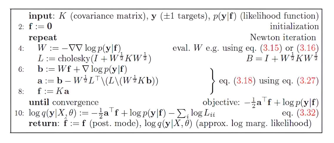
图 1.算法 3.1 用于搜索 f_hat 和 LML 模式
- 该过程首先计算 K 核协方差矩阵。为了更快、更稳定地收敛,将前一次超参数优化迭代的 mu_f_train 结果用作 f 的初始猜测,而不是每次从零向量开始。
- 使用牛顿法迭代更新 f_hat。
- 计算 NLML:当模式 f 收敛后(当 LML 的变化小于 m_tolerance 时),我们将 NLML 值传递给优化器。
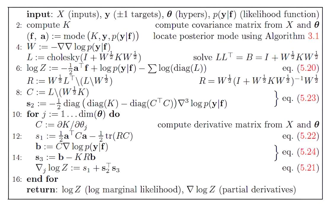
图 2.算法 5.1 计算 LML 梯度
- 核超参数上的梯度涉及 R 和 C 辅助矩阵的计算。使用 cho_solve 计算 R 矩阵,使用 LinearEquationsSolutionTriangular 计算 C 矩阵。
- 潜在函数的后验协方差矩阵基于训练数据 Σf_train = K−C^TC 计算得到。
- 每个核超参数(dK_dtheta_j)的梯度由显式部分(s1)和隐式部分(s2、s3)组成。s1 的计算通过使用 DiagonalTrace 进行优化,s3 还包括用于求解系统的 cho_solve。
- 利用对数似然函数及其 Hessian 矩阵对相应超参数的导数来计算关于似然超参数的梯度。为此,使用了 “likelihood” 对象的 LogLikelihoodGradientParam 和 LogLikelihoodHessianDerivative 方法。
现在我们已经有了所有基本构建模块(核函数、似然函数、推断方法),接下来让我们演示一下该库是如何工作的。
在合成数据上测试库
Gpsynthetic.mq5 脚本将帮助我们使用简单的合成数据测试我们的库。这将使我们能够确保实现的方法是有效和正确的。
// --- Include the GP library ---
#include <GP/GP.mqh>

enum IntervalType
  {
   INTERVAL_F = 0, // Confidence interval of the f* latent function
   INTERVAL_Y = 1  // Confidence interval of y* observations
  };

enum Type_inference
  {
   Exact = 0,   // Exact Inference
   Laplace = 1  // Laplace Inference
  };

enum Type_Data
  {
   Regression = 0,    // Regression
   Classification = 1 // Classification
  };

//--- Input parameters
input IntervalType    interval_type  = INTERVAL_F;    // Interval type to display
input Type_Data       DataType       = Classification;
input Type_inference  inf            = Laplace ;        // Inference type

//+------------------------------------------------------------------+
//| Script program start function                                    |
//+------------------------------------------------------------------+
void OnStart()
  {
   string InpFileName1;
   string InpFileName2;
   string InpFileName3;
   string InpFileName4;

   if(DataType == Regression)
     {
      // Regression data
      InpFileName1 = "Data_Regression/X_train.csv";
      InpFileName2 = "Data_Regression/Y_train.csv";
      InpFileName3 = "Data_Regression/X_test.csv";
      InpFileName4 = "Data_Regression/Y_test.csv";
     }
   else
     {
      InpFileName1 = "Data_Classification/X.csv";  // 200
      InpFileName2 = "Data_Classification/y.csv";
      InpFileName3 = "Data_Classification/X_star.csv";
      InpFileName4 = "Data_Classification/y_star.csv";
     }

//----------- Dataset
   matrix x_train, y_train, x_test, y_test;
   CSVtoMatrix(InpFileName1,x_train);
   CSVtoMatrix(InpFileName2,y_train);
   CSVtoMatrix(InpFileName3,x_test);
   CSVtoMatrix(InpFileName4,y_test);

// Create label vectors from matrices
   vector y_train_ = y_train.Col(0);
   vector y_test_ = y_test.Col(0);

//--- 1. Create kernel objects
   IKernel* rbf = new RBFKernel(1,1);
// IKernel* linear = new LinearKernel(1.0);
// IKernel* periodic = new PeriodicKernel(1.0, 1.0, 5.8);

//--- 2. Combination of kernels (creation of a compound kernel)
// IKernel* functional_kernels_array[] = {rbf, linear, periodic};
// SumKernel* combined_functional_kernel = new SumKernel(functional_kernels_array);

//--- 3. Creating a likelihood object
   ILikelihood* likelihood = NULL; // Declare a pointer of the base type

   if(DataType == Regression)
     {
      likelihood = new GaussianLikelihood(1); // Assign the object
     }

   if(DataType == Classification)
     {
      likelihood = new LogitLikelihood();
     }

//--- 4. Create the inference object
   IInference* inference; // Declare a pointer to the interface
// Select the inference type:
   if(inf == Exact)
     {
      inference = new ExactInference();
     }
   else
     {
      inference = new LaplaceInference(100, 1e-10);
     }

//--- 5. Create an instance of the Gaussian Process model
   CREATE_GP_MODEL(gp_model, rbf, likelihood, inference,x_train, y_train_);
//  CREATE_GP_MODEL(gp_model, combined_functional_kernel, likelihood, inference,x_train, y_train_);
//--------------------------------------------------

   ulong start_time_fit = GetMicrosecondCount();
//--- 6. Hyperparameter optimization
   gp_model.Fit();
   ulong end_time_fit = GetMicrosecondCount();
   double elapsed_time_ms = (end_time_fit - start_time_fit) / 1000.0;
   Print(inference.GetName());
   Print("Fit execution time: ", StringFormat("%.3f", elapsed_time_ms), " ms");
   gp_model.PrintOptimizedKernelParameters();

//--- 7. Forecast for test points
   GPPredictionResult gp_predictions; // create a structure where the prediction results are to be set
   ulong start_time_predict = GetMicrosecondCount();
   gp_model.Predict(x_test, gp_predictions,PROBIT); // MONTE_CARLO,NUM_INTEGR,PROBIT
   ulong end_time_predict = GetMicrosecondCount();
   elapsed_time_ms = (end_time_predict - start_time_predict) / 1000.0;
   Print("Predict execution time: ", StringFormat("%.3f", elapsed_time_ms), " ms");

// --- 8. Classification results
   if(DataType == Classification)
     {
      DisplayClassificationResults(gp_predictions, y_test_);
     }
//--- 9. Regression Results
   if(DataType == Regression)
     {
      VisualizeGP(x_train, y_train, x_test, y_test_, gp_predictions, gp_model, 15);
     }

//--- 10. Releasing memory
   delete gp_model;
  }
根据所选的数据类型(回归或分类),脚本确定包含训练和测试数据的 CSV 文件的路径。这些文件假定位于 “Files” 目录下的 “Data_Regression” 或 “Data_Classification” 文件夹中。
接下来,创建核函数对象。要构建更复杂的协方差函数,可以使用 SumKernel 或 ProductKernel 等组合核函数。
然后,根据所选的数据类型创建似然函数对象(ILikelihood)以及推理对象(IInference)。
使用 CREATE_GP_MODEL 宏(或类似的构造函数),创建一个 GP 模型,该模型将选定的核函数、似然函数和推断方法与训练数据关联起来。
gp_model.Fit(int maxiter = 20) 方法启动模型训练过程。该方法现在新增了一个参数,用于设置 “maxiter” 迭代的最大次数。
训练完成后,使用 gp_model.Predict() 方法对新的(测试)数据 x_test 进行预测。预测结果(均值、协方差、概率/标签)存储在 GPPredictionResult 结构中。
对于分类,您可以选择预测模式(PROBIT、NUM_INTEGR、MONTE_CARLO)。
然后,脚本会输出预测结果:
- 对于分类,调用 DisplayClassificationResults() 函数,该函数计算准确率指标和预测概率;
- 对于回归分析 — VisualizeGP() 函数负责呈现结果。
回归示例使用由函数 y = sin(x) + 0.5 * x + noise(sigma = 0.1) 生成的合成数据。我们不会详细讨论这个问题,因为我们在专门讨论回归的文章中已经讨论过了。请注意,自从我们改用 OpenBLAS 库中的解析梯度和方法以来,训练时间已经大大缩短了。
对于二元分类,使用代表 XOR(异或)问题的数据。这是机器学习中的一个经典问题,它证明了线性模型的局限性以及使用非线性方法(如 GP)的必要性。
回想一下,异或运算是一种逻辑运算,它接受两个二进制输入(0 或 1),如果其中一个输入为 1,则返回 1,否则返回 0。异或真值表:
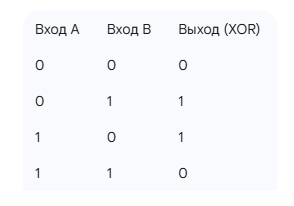
二元 XOR 分类的任务是构建一个模型,给定两个输入(A,B),预测它们的 XOR 输出(0 和 1)。但由于我们的模型只适用于 +1 和 -1 标签,我们将把 0 标签替换为 -1。
XOR 问题的数据生成方式如下。二维输入点 X(X=[x1,x2]),它们在一定范围内随机分布(例如每个轴上的 [-4,4])。这些点的 y 标签是基于 XOR 逻辑确定的:
- 如果 x1 和 x2 两个数的符号相同(均为正或均为负),则它们的乘积为 x1⋅x2 将会是正的。在这种情况下,标签被赋予 +1。
- 如果 x1 和 x2 它们的符号不同(一个为正,另一个为负),则它们的乘积为 x1⋅x2 结果将为负。在这种情况下,标签被赋予-1。
因此,点 (+,+) 和 (−,−) 属于 +1 类,点 (+,−) 和 (−,+) 属于 −1 类。对于这个任务,我们将只使用 RBF 核,因为它很好地处理了非线性依赖关系,允许高斯过程有效地分离这些类。
在测试过程中,我使用了 200 个观察值进行训练,并使用了 100 个新点来测试准确性。预测准确率达到 98%,这表明 GP 在解决非线性分类问题方面具有很高的效率。
GPRegressor 指标:基于 GP 的时间回归
该指标是考虑不确定性的金融时间序列动态预测的一个例子。通过使用滑动窗口形成训练样本并不断对模型进行再训练,它实现了适应不断变化的市场条件的原则。
//+------------------------------------------------------------------+
//|                                                  GPRegressor.mq5 |
//|                                                           Eugene |
//|                                             https://www.mql5.com |
//+------------------------------------------------------------------+
#property copyright "Eugene"
#property link      "https://www.mql5.com"
#property version   "1.00"
// --- Include the GP library ---
#include <GP/GP.mqh>

#property indicator_chart_window
#property indicator_buffers 3
#property indicator_plots   2

// plot Predicted mean
#property indicator_label1  "Predicted mean"
#property indicator_type1   DRAW_LINE
#property indicator_color1  clrBlue
#property indicator_style1  STYLE_SOLID
#property indicator_width1  2

//--- plot Confidence interval
#property indicator_label2  "Confidence interval"
#property indicator_type2   DRAW_FILLING
#property indicator_color2   clrLightGray
#property indicator_width2  1

//--- Input parameters
input int    WindowLength   = 10;    // Window length for training the model
input int    calculate_bars = 100;   // History depth for calculation
input double zscore         = 1.96;  // z value for the interval (1.96 = 95%)
input bool   ShowRMSE       = false; // Show RMSE metric

//--- Buffers variables for rendering
double  ExtPredictionBuffer[]; // Buffer for predicted values
double  ExtUpperBandBuffer[];  // Buffer for the upper border of the confidence interval
double  ExtLowerBandBuffer[];  // Buffer for the lower border

//--- Global objects
GaussianProcess* g_gp_model       = NULL;
IKernel*         g_kernel         = NULL;
ILikelihood*     g_likelihood     = NULL;
IInference*      g_inference      = NULL;

//--- Global matrix for X_train temporary indices
matrix g_X_train;
//--- Global variables for RMSE data accumulation
vector gp_pred;
vector naive_pred;
vector y_true;
// Flag indicating whether the RMSE has already been calculated (for a one-time calculation)
bool rmse_calculated = false;
string comment;
double gp_rmse,naive_rmse;
//+------------------------------------------------------------------+
//| Custom indicator initialization function                         |
//+------------------------------------------------------------------+
int OnInit()
  {
   if(Bars(Symbol(), Period()) < WindowLength + calculate_bars)
     {
      PrintFormat("Error: Not enough bars to calculate. Minimum %d required. Available: %d",
                  WindowLength + calculate_bars, Bars(Symbol(), Period()));
      return(INIT_FAILED);
     }

   rmse_calculated = false; // Reset the flag on initialization/reinitialization
//--- Initialize global vectors for RMSE
   gp_pred.Resize(calculate_bars-1);
   naive_pred.Resize(calculate_bars-1);
   y_true.Resize(calculate_bars-1);

//--- indicator buffers mapping
   SetIndexBuffer(0, ExtPredictionBuffer, INDICATOR_DATA);
   SetIndexBuffer(1, ExtUpperBandBuffer,  INDICATOR_DATA);
   SetIndexBuffer(2, ExtLowerBandBuffer,  INDICATOR_DATA);

//--- Create kernel, likelihood, and inference method objects
   g_kernel = new RBFKernel(1.0, 1.0);
   if(g_kernel == NULL)
     {
      Print("Failed to create RBFKernel object");
      return(INIT_FAILED);
     }

   g_likelihood = new GaussianLikelihood(0.1);
   if(g_likelihood == NULL)
     {
      Print("Failed to create GaussianLikelihood object");
      delete g_kernel;
      return(INIT_FAILED);
     }

   g_inference = new ExactInference();
   if(g_inference == NULL)
     {
      Print("Failed to create ExactInference object");
      delete g_kernel;
      delete g_likelihood;
      return(INIT_FAILED);
     }

//--- Initialize the feature matrix X_train (one feature - time)
   g_X_train = matrix::Zeros(WindowLength, 1);
   for(int i = 0; i < WindowLength; i++)
     {
      g_X_train[i][0] = (double)(i + 1); // X = [1, 2, ..., WindowLength]
     }

//--- Create the GaussianProcess object
// Pass g_X_train and empty y_train
   vector initial_y_train = vector::Zeros(WindowLength);
   g_gp_model = new GaussianProcess(g_kernel, g_likelihood, g_inference, g_X_train, initial_y_train);
   if(g_gp_model == NULL)
     {
      Print("Failed to create GaussianProcess object");
      delete g_kernel;
      delete g_likelihood;
      delete g_inference;
      return(INIT_FAILED);
     }
   return(INIT_SUCCEEDED);
  }

//+------------------------------------------------------------------+
//|                                                                  |
//+------------------------------------------------------------------+
int OnCalculate(const int32_t rates_total,
                const int32_t prev_calculated,
                const datetime &time[],
                const double &open[],
                const double &high[],
                const double &low[],
                const double &close[],
                const long &tick_volume[],
                const long &volume[],
                const int32_t &spread[])
  {
// Check for sufficient number of bars
   if(rates_total < WindowLength)
     {
      Print("Error: Not enough bars to calculate. At least ", WindowLength, " is required, available: ", rates_total);
      return(0);
     }

   int start;
   if(prev_calculated == 0)
     {
      // Determine where to start the calculation.
      // calculate_bars - history depth to calculate.
      // MathMax(WindowLength, ...) ensures that we start no sooner than there is a full window of data.
      start = MathMax(WindowLength, rates_total - calculate_bars);
      // Initialize all buffers with EMPTY_VALUE
      ArrayInitialize(ExtPredictionBuffer, EMPTY_VALUE);
      ArrayInitialize(ExtUpperBandBuffer,  EMPTY_VALUE);
      ArrayInitialize(ExtLowerBandBuffer,  EMPTY_VALUE);
      // Set the start of rendering buffers
      PlotIndexSetInteger(0, PLOT_DRAW_BEGIN, start);
      PlotIndexSetInteger(1, PLOT_DRAW_BEGIN, start);
      PlotIndexSetInteger(2, PLOT_DRAW_BEGIN, start);
     }
   else
     {
      if(time[rates_total - 1] == time[prev_calculated - 1])
        {
         // This means that a new bar has NOT appeared.
         // We are on the same bar, just new ticks have arrived.
         return(rates_total);
        }
      // If the time of the last bar has changed, then a new closed bar has appeared.
      // Start calculation from prev_calculated to handle all new bars.
      start = prev_calculated;
     }

   for(int i = start; i < rates_total && !IsStopped(); i++)
     {
      // Check if there are enough bars to form a window
      if(i < WindowLength)
        {
         Print("Error: Not enough bars to form a window on bar ", i, ". Required: ", WindowLength, ", available: ", i);
         ExtPredictionBuffer[i] = EMPTY_VALUE;
         ExtUpperBandBuffer[i]  = EMPTY_VALUE;
         ExtLowerBandBuffer[i]  = EMPTY_VALUE;
         continue; // Skip this bar
        }

      // Form y vector from close[i-1], close[i-2], ..., close[i-WindowLength]
      // close[i-1]               - the newest bar in the window
      // close[i-WindowLength] - the oldest bar in the window
      vector y(WindowLength);
      for(int j = 0; j < WindowLength; j++)
        {
         y[WindowLength - 1 - j] = close[i - 1 - j];
        }
      //Print(" y = ", y[WindowLength-1]); // The newest bar in the window

      //--- Data standardization
      double mu_raw = y.Mean();
      // Print("mu_raw = ", mu_raw);
      double sigma_raw = y.Std();
      // Print("sigma_raw = ", sigma_raw);
      vector y_standardized = (y - mu_raw) / sigma_raw;

      //---  Set up training data
      g_gp_model.SetTrainingData(g_X_train, y_standardized);

      //--- Reset initial hyperparameters before Fit()
      vector initial_params(3);
      initial_params[0] = 1.0; // sigma_f (RBFKernel)
      initial_params[1] = 1.0; // length_scale (RBFKernel)
      initial_params[2] = 0.1; // sigma_n (GaussianLikelihood)
      g_gp_model.SetHyperparameters(initial_params);
      // vector params =  g_gp_model.GetCurrentHyperparameters();
      // Print(params);

      // ulong start_time_fit = GetMicrosecondCount();
      //--- Train the model
      if(!g_gp_model.Fit())
        {
         Print("Error: Failed to optimize GP hyperparameters for bar ", i);
         ExtPredictionBuffer[i] = EMPTY_VALUE;
         ExtUpperBandBuffer[i]  = EMPTY_VALUE;
         ExtLowerBandBuffer[i]  = EMPTY_VALUE;
         continue; // Skip the current bar
        }
      //ulong end_time_fit = GetMicrosecondCount();
      // double elapsed_time_ms = (end_time_fit - start_time_fit) / 1000.0;
      //Print("Fit execution time: ", StringFormat("%.3f", elapsed_time_ms), " мс");

      vector params =  g_gp_model.GetCurrentHyperparameters();
      double sigma_f      = params[0]; // sigma_f (RBFKernel)
      double length_scale = params[1]; // length_scale (RBFKernel)
      double sigma_n      = params[2]; // sigma_n (GaussianLikelihood)


      // --- Create a point for forecasting (X_star)
      // Predict the value for the next step after WindowLength
      matrix X_star = matrix::Zeros(1, 1);
      X_star[0][0] = (double)(WindowLength + 1);

      // --- Perform the prediction
      GPPredictionResult gp_predictions;
      if(!g_gp_model.Predict(X_star, gp_predictions))
        {
         Print("Error: Failed to get forecast from GP model for bar ", i);
         ExtPredictionBuffer[i] = EMPTY_VALUE;
         ExtUpperBandBuffer[i]  = EMPTY_VALUE;
         ExtLowerBandBuffer[i]  = EMPTY_VALUE;
         continue;
        }

      // ---
      double predicted_mean_st = gp_predictions.mu_f_star[0];
      // --- Perform the inverse transformation of the predicted mean value
      // back to the original price scale
      double predicted_mean = predicted_mean_st * sigma_raw + mu_raw;

      double sigma_f_star = gp_predictions.Sigma_f_star[0,0]; // dispersion (Σ) of f* signal
      double predicted_variance_st = gp_predictions.Sigma_y_star[0,0]; // dispersion(Σ) of y* observation
      // --- Perform the inverse dispersion transformation
      // The variance is scaled by the square of the standard deviation (sigma_raw) of the data,
      // used for standardization.
      double predicted_variance = predicted_variance_st * sigma_raw * sigma_raw;

      // Calculate the predicted confidence interval
      double std_predict = MathSqrt(predicted_variance);
      double upper_bound = predicted_mean + zscore * std_predict;
      double lower_bound = predicted_mean - zscore * std_predict;

      // --- Save the results to the indicator buffers for rendering
      ExtPredictionBuffer[i] = predicted_mean;
      ExtUpperBandBuffer[i]  = upper_bound;
      ExtLowerBandBuffer[i]  = lower_bound;

      comment = StringFormat("GP Regressor | Mean=%.5f | Upper=%.5f | Lower=%.5f |\n",
                             predicted_mean, upper_bound, lower_bound);
      comment+= StringFormat("Sigma_f = %.5f | Length_Scale = %.5f | Sigma_n = %.5f\n",sigma_f,length_scale,sigma_n);
      comment+= StringFormat("mu f* = %.5f | Σ y* = %.5f | Σ f*= %.5f",predicted_mean_st,predicted_variance_st,sigma_f_star);
      Comment(comment);
      // Debug output
      Print("Bar forecast ", i, ": Mean=", DoubleToString(predicted_mean, Digits()),
            " Upper=", DoubleToString(upper_bound, Digits()),
            " Lower=", DoubleToString(lower_bound, Digits()));
     }

// ---  Calculate RMSE to evaluate the efficiency of the GP forecast model compared to a simple "naive" forecast
   if(ShowRMSE && !rmse_calculated)
     {
      vector returns(calculate_bars-1);
      for(int j=0; j <calculate_bars-1;j++)
        {
         // true value
         y_true[j] = close[rates_total - calculate_bars + j];
         //Print("y_true[j]", y_true[j] );

         // GP forecast:
         gp_pred[j] = ExtPredictionBuffer[rates_total-calculate_bars + j];
         //Print("gp_pred[j]", gp_pred[j] );

         // "Naive" forecast (price tomorrow = price today):
         naive_pred[j] = close[rates_total - calculate_bars + j-1];
         // Print("naive_pred[j]", naive_pred[j] );

         returns[j] = close[rates_total - calculate_bars + j]  - close[rates_total - calculate_bars + j-1];
        }

      gp_rmse=gp_pred.RegressionMetric(y_true,REGRESSION_RMSE);
      naive_rmse=naive_pred.RegressionMetric(y_true,REGRESSION_RMSE);
      double std_returns = returns.Std(); // standard deviation of Close increments
      comment = comment + StringFormat("\nRMSE GP: %.5f | RMSE Naive: %.5f | StdDev Returns Close: %.5f ", gp_rmse, naive_rmse, std_returns);
      rmse_calculated = true;
     }
   Comment(comment);
//--- Return rates_total for the next call
   return(rates_total);
  }
//+------------------------------------------------------------------+
//| Custom indicator deinitialization function                       |
//+------------------------------------------------------------------+
void OnDeinit(const int reason)
  {
//--- Clear the comment on the chart
   Comment("");
//--- Free up the allocated memory for the GP object
   if(g_gp_model != NULL)
     {
      delete g_gp_model;
     }
  }
//+------------------------------------------------------------------+
输入:
- WindowLength — 用于训练 GP 模型的数据窗口长度(以 K 线数为单位)。
- calculate_bars — 用于计算和绘制指标的历史深度。
- zscore — 构建置信区间的标准差数量(例如,95% 的置信区间为 1.96)。
- ShowRMSE — 用于显示预测的均方根误差 (RMSE) 的标志。
初始化(OnInit):
- 全局对象。创建并初始化全局核对象(RBFKernel)、似然函数(GaussianLikelihood)和推断方法(ExactInference)。
- X_train 特征。GPRegressor 使用训练窗口内的时间索引(从 1 到 WindowLength)作为 X 输入,实现随时间变化的回归。
- GaussianProcess 模型。g_gp_model 对象使用指定的组件进行初始化,而 y_train 最初为空,需要动态填充。
主计算循环(OnCalculate):
- 数据生成:在每根 K 线上,提取最新收盘价的窗口长度,以生成 y 向量。
- 数据标准化:为了保证 GP 运算的数值稳定性,y 被标准化(均值为零,方差为 1)。
- 更新和训练模型:
- 每次训练前,超参数都会重置为初始值(g_gp_model.SetHyperparameters)
- GP 模型在当前标准化价格窗口上进行训练 g_gp_model.Fit()。
- 预测:为了预测下一根 K 线,创建时间索引为 WindowLength + 1 的 X_star 点。g_gp_model.Predict() 方法执行预测,返回标准化数据的均值(mu_f_star)和方差(Sigma_y_star)。
- 去标准化:使用当前窗口的均值(mu_raw)和标准差(sigma_raw),将预测的均值和方差转换回原始价格尺度。
- 置信区间:使用用户指定的 zscore 标准偏差值,根据转换后的平均值和标准偏差计算区间的上限和下限。
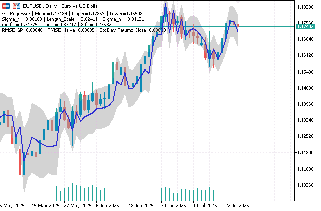
图 3.回归模型预测及 95% 置信区间
计算 RMSE 指标:
该指标显示 GP 模型预测的 RMSE 统计数据,以及每个用户请求的最后一个计算基数的 “Naive”(朴素) 预测(其中明天的价格=今天的价格)。它有助于客观地评估当前模型的效率。
例如,EURUSD 在分钟时间周期内的典型指标可能包括:RMSE GP (0.00032) | RMSE Naive (0.00029),收盘价增量的标准差 (StdDev Returns Close) 为 0.00029。
GP RMSE 高于 Naive RMSE 的事实表明,在给定的分析期内,GP 模型的表现不如简单的朴素预测。此外,RMSE Naive 和 StdDev Returns Close 相等是随机游走的特征,其中未来的价格变化与过去的价格变化无关,而当前值是最佳预测。
由此我们可以得出结论,在时间序列的这一部分中,要么没有可预测的模式,要么当前 GP 模型配置(仅使用时间作为特征)还无法提取有用的信息来超越简单的预测。
GPClassifier 指标:基于高斯过程的分类
GPClassifier 指标展示了在二元分类问题中创建、训练和预测 GP 模型的过程。所使用的特征是收盘价的增量,这些增量是在历史数据的滑动窗口中计算出来的。NormalizeData 函数用于对特征矩阵进行归一化,以稳定模型训练。
//+------------------------------------------------------------------+
//|                                                 GPClassifier.mq5 |
//|                                                           Eugene |
//|                                             https://www.mql5.com |
//+------------------------------------------------------------------+
#property copyright "Eugene"
#property link       "https://www.mql5.com"
#property version    "1.00"
// --- Include the GP library ---
#include <GP/GP.mqh>

#property indicator_chart_window
#property indicator_buffers 4
#property indicator_plots   2

// plot for predicted class "+1" (up arrows)
#property indicator_label1  "Predicted Class +1"
#property indicator_type1   DRAW_ARROW
#property indicator_color1  clrGreen
#property indicator_width1  1

// plot for predicted class "-1" (down arrows)
#property indicator_label2  "Predicted Class -1"
#property indicator_type2   DRAW_ARROW
#property indicator_color2  clrBlack
#property indicator_width2  1

//--- Input parameters
input int       WindowLength         = 10;    // Window length for training the GP model
input int       NumLags              = 1;     // Number of features
input int       calculate_bars       = 100;   // History depth for calculation
input double    ProbabilityThreshold = 0.5;   // Probability threshold
input int       ArrowShiftPx         = 10;    // Arrow offset in pixels
input bool      ShowACCURACY         = false; // Show accuracy on the chart

//--- Buffers variables for rendering
double  ExtClassUpBuffer[];              // Buffer for displaying UP arrows
double  ExtClassDownBuffer[];            // Buffer for displaying DOWN arrows
double  ExtPredictedClassBuffer[];       // Buffer for storing predicted class labels
double  ExtPredictedProbabilityBuffer[]; // Buffer for storing predicted probabilities

//--- Global Gaussian process objects
GaussianProcess* g_gp_model    = NULL;
IKernel*         g_kernel      = NULL;
ILikelihood*     g_likelihood  = NULL;
IInference*      g_inference   = NULL;

//--- Global variables for classification metrics
bool accuracy_calculated = false;
vector gp_pred,naive_pred,y_true,gp_accuracy,naive_accuracy;
string comment;
int currentsize;
//+------------------------------------------------------------------+
//| Custom indicator initialization function                         |
//+------------------------------------------------------------------+
int OnInit()
  {
   accuracy_calculated = false; // Reset the flag on initialization/reinitialization
//--- Initialize global vectors for Accuracy
   gp_pred.Resize(0);
   naive_pred.Resize(0);
   y_true.Resize(0);
   gp_accuracy.Resize(1);
   naive_accuracy.Resize(1);
   currentsize = 0;
//--- indicator buffers mapping
   SetIndexBuffer(0, ExtClassUpBuffer,     INDICATOR_DATA);    // For up arrows
   SetIndexBuffer(1, ExtClassDownBuffer,   INDICATOR_DATA);    // For down arrows
   SetIndexBuffer(2, ExtPredictedClassBuffer, INDICATOR_CALCULATIONS); //  to store predicted labels
   SetIndexBuffer(3, ExtPredictedProbabilityBuffer, INDICATOR_CALCULATIONS); // to store probabilities
// --- Set arrow symbols
   PlotIndexSetInteger(0, PLOT_ARROW, 225);   // Up arrow for buffer 0
   PlotIndexSetInteger(1, PLOT_ARROW, 226);   // Down arrow for buffer 1
// --- Set the arrow offset in pixels ---
// For the up arrows (buffer 0), use a negative offset so they are above High
   PlotIndexSetInteger(0, PLOT_ARROW_SHIFT, -ArrowShiftPx); // negative = up
// For the down arrows (buffer 1), use a positive offset so they are below Low
   PlotIndexSetInteger(1, PLOT_ARROW_SHIFT, ArrowShiftPx); // positive = down

// Add a check for the ratio of NumLags and WindowLength
   if(NumLags <= 0)
     {
      Print("Error: NumLags must be positive number");
      return(INIT_FAILED);
     }
   if(NumLags >= WindowLength)
     {
      Print("Error: NumLags (", NumLags, ") cannot exceed or be equal to WindowLength (", WindowLength, ").");
      return(INIT_FAILED);
     }

//--- Create kernel, likelihood, and inference method objects
   g_kernel = new RBFKernel(1.0, 1.0);
   if(g_kernel == NULL)
     {
      Print("Failed to create RBFKernel object");
      return(INIT_FAILED);
     }

   g_likelihood = new LogitLikelihood();
   if(g_likelihood == NULL)
     {
      Print("Failed to create LogitLikelihood object");
      delete g_kernel;
      return(INIT_FAILED);
     }

   g_inference = new LaplaceInference();
   if(g_inference == NULL)
     {
      Print("Failed to create ExactInference object");
      delete g_kernel;
      delete g_likelihood;
      return(INIT_FAILED);
     }
// --- Create the GaussianProcess model
// Pass empty matrices for X_train and y_train.
// They will be overridden in OnCalculate.
   g_gp_model = new GaussianProcess(g_kernel, g_likelihood, g_inference,matrix::Zeros(1,1), vector::Zeros(1));
   if(g_gp_model == NULL)
     {
      Print("Failed to create GaussianProcess object");
      delete g_kernel;
      delete g_likelihood;
      delete g_inference;
      return(INIT_FAILED);
     }
   return(INIT_SUCCEEDED);
  }
//+------------------------------------------------------------------+
//| Custom indicator iteration function                              |
//+------------------------------------------------------------------+
int OnCalculate(const int32_t rates_total,
                const int32_t prev_calculated,
                const datetime &time[],
                const double &open[],
                const double &high[],
                const double &low[],
                const double &close[],
                const long &tick_volume[],
                const long &volume[],
                const int32_t &spread[])
  {
// Check for sufficient number of bars
   if(rates_total < WindowLength + NumLags + 1)
     {
      Print("Error: Not enough bars to calculate. Required at least ", WindowLength + NumLags + 1, ", available: ", rates_total);
      return(0);
     }

   int start;
   if(prev_calculated == 0)
     {
      start = MathMax(WindowLength + NumLags + 1, rates_total - calculate_bars);
      // Initialize all EMPTY_VALUE buffers
      ArrayInitialize(ExtClassUpBuffer, EMPTY_VALUE);
      ArrayInitialize(ExtClassDownBuffer, EMPTY_VALUE);
      // Number of initial bars without rendering and values in DataWindow
      PlotIndexSetInteger(0, PLOT_DRAW_BEGIN, start);
      PlotIndexSetInteger(1, PLOT_DRAW_BEGIN, start);
     }
   else
     {
      if(time[rates_total - 1] == time[prev_calculated - 1])
        {
         return(rates_total);
        }
      start = prev_calculated;
     }

// --- Main forecast calculation loop
   for(int i = start; i < rates_total && !IsStopped(); i++)
     {
      // Check if there are enough bars to form X and y window
      if(i < WindowLength + NumLags + 1)
        {
         ExtClassUpBuffer[i] = EMPTY_VALUE;
         ExtClassDownBuffer[i] = EMPTY_VALUE;
         continue;
        }

      // --- Step 1: Generate training data (X_train and y_train)
      matrix X_train = matrix::Zeros(WindowLength, NumLags);
      vector y_train = vector::Zeros(WindowLength);

      for(int j = 0; j < WindowLength; j++)
        {
         // Calculate the bar index in the 'close' array for the current observation in the window.
         int idx = i - WindowLength + j;
         // Formation of features (lags) for the current observation (X_train[j] strings)
         for(int lag_idx = 0; lag_idx < NumLags; lag_idx++)
           {
            // Example:
            // lag_idx = 0: (close[idx - 1] - close[idx - 2]) - increment of the previous bar
            // lag_idx = 1: (close[idx - 2] - close[idx - 3]) - increment of the bar before last
            X_train[j,lag_idx] = close[idx - 1 - lag_idx] - close[idx - 2 - lag_idx];
           }

         // Y_train[j]: Binary label for price increment on idx bar.
         if(close[idx] - close[idx - 1] > 0)
           {
            y_train[j] = 1; // Price increased
           }
         else
           {
            y_train[j] = -1; // Price decreased or remained unchanged
           }

        }
      // Print(y_train);

      // --- Normalize X_train
      matrix X_train_norm;
      vector out_mean;
      vector out_std;
      if(!NormalizeData(X_train,X_train_norm,out_mean,out_std))
        {
         Print("Error: Failed to normalize feature matrix ", i);
         continue;
        }

      // --- Step 2: Feed data into the GP model
      g_gp_model.SetTrainingData(X_train_norm, y_train);

      // Reset initial hyperparameters before each Fit() training
      vector initial_params(2);
      initial_params[0] = 1.0; // sigma_f (RBFKernel)
      initial_params[1] = 1.0; // length_scale (RBFKernel)
      g_gp_model.SetHyperparameters(initial_params);

      // --- Step 3: Train the model
     //  ulong start_time_fit = GetMicrosecondCount();
      if(!g_gp_model.Fit())
        {
         Print("Error: Failed to optimize GP hyperparameters for bar ", i);
         ExtClassUpBuffer[i] = EMPTY_VALUE;
         ExtClassDownBuffer[i] = EMPTY_VALUE;
         continue;
        }
       // ulong end_time_fit = GetMicrosecondCount();
      //  double elapsed_time_ms = (end_time_fit - start_time_fit) / 1000.0;
       // Print("Fit execution time: ", StringFormat("%.3f", elapsed_time_ms), " ms");

      // --- Step 4: Create a point for the X_star forecast
      // X_star - increment of prices of previous NumLags closed bars,
      // used to predict the movement of the current bar (i bar).
      matrix X_star = matrix::Zeros(1, NumLags);
      for(int lag_idx = 0; lag_idx < NumLags; lag_idx++)
        {
         X_star[0][lag_idx] = close[i - 1 - lag_idx] - close[i - 2 - lag_idx];
        }
      //  X_star should also be normalized using the same means and standard deviations,
      //  as for the corresponding X_train columns.
      for(int lag_idx = 0; lag_idx < NumLags; lag_idx++)
        {
         X_star[0][lag_idx] = (X_star[0][lag_idx] - out_mean[lag_idx]) / out_std[lag_idx];
        }

      // --- Step 5: Perform the prediction
      GPPredictionResult gp_predictions;
      if(!g_gp_model.Predict(X_star, gp_predictions))
        {
         Print("Error: Failed to get forecast from GP model for bar ", i);
         ExtClassUpBuffer[i] = EMPTY_VALUE;
         ExtClassDownBuffer[i] = EMPTY_VALUE;
         continue;
        }

      double predicted_probability = gp_predictions.predicted_probabilities[0]; // Probability for a single test point
      int predicted_class = (int)gp_predictions.predicted_labels[0]; // Label (+1 or -1)

      // --- Step 6: Save the results to the indicator buffers for rendering
      ExtClassUpBuffer[i] = EMPTY_VALUE;
      ExtClassDownBuffer[i] = EMPTY_VALUE;
      ExtPredictedClassBuffer[i] = predicted_class;
      ExtPredictedProbabilityBuffer[i] = predicted_probability;

      // Add the probability output and the number of features (lags) as a chart comment
      comment = StringFormat("GP Classifier (Lags: %d) | Probability(UP) = %.10f", NumLags, predicted_probability);
      Comment(comment);

      // If the predicted class is "+1" and the probability is above the given threshold
      if(predicted_class == 1 && predicted_probability > ProbabilityThreshold)
        {
         ExtClassUpBuffer[i] = high[i];
        }
      // If the predicted class is "-1" and the probability is above the given threshold
      else
         if(predicted_class == -1 && (1.0 - predicted_probability) > ProbabilityThreshold)
           {
            ExtClassDownBuffer[i] = low[i];
           }

      Print("Bar forecast ", i, ": Probability(UP)=" + DoubleToString(predicted_probability, 10) +
            ", Predicted Class=" + IntegerToString(predicted_class), " time: ", time[i]);
     }

// --- Calculate classification accuracy for assessing the efficiency of the GP predictive model in comparison
//with a "naive" forecast.
   if(ShowACCURACY  && !accuracy_calculated)
     {
      for(int j=0; j <calculate_bars-1;j++)
        {
         // index to the current bar
         int bar_idx = rates_total - calculate_bars + j;

         if(ExtClassUpBuffer[bar_idx]!= EMPTY_VALUE || ExtClassDownBuffer[bar_idx] != EMPTY_VALUE)
           {
            currentsize = (int)gp_pred.Size();
            currentsize++;
            gp_pred.Resize(currentsize,100);
            naive_pred.Resize(currentsize,100);
            y_true.Resize(currentsize,100);

            // True label: count to the current bar
            if(close[bar_idx] - close[bar_idx - 1] > 0)
              {
               y_true[currentsize-1] = 1; // Price increased
              }
            else
              {
               y_true[currentsize-1] = -1; // Price decreased or remained unchanged
              }
            // Print("y_true",  y_true[currentsize-1] );

            // GP forecast: count to the current bar
            gp_pred[currentsize-1] = ExtPredictedClassBuffer[bar_idx];
            // Print(" gp_pred",  gp_pred[currentsize-1]);

            // "Naive" forecast: the "for tomorrow" bar label is equal to the "today" label
            if(close[bar_idx - 1] - close[bar_idx - 2] > 0)
              {
               naive_pred[currentsize-1] = 1;
              }
            else
              {
               naive_pred[currentsize-1] = -1;
              }
           }

        }

      if(!(int)gp_pred.Size()==0)
        {
         gp_accuracy=gp_pred.ClassificationMetric(y_true,CLASSIFICATION_ACCURACY);
         naive_accuracy=naive_pred.ClassificationMetric(y_true,CLASSIFICATION_ACCURACY);
         comment += StringFormat("\nGP Accuracy: %.2f %% | Naive Accuracy: %.2f %%", gp_accuracy[0], naive_accuracy[0]);
         comment += StringFormat("\nNumber of Filtered Signals: %d", (int)gp_pred.Size());
        }
      else
        {
         comment += StringFormat("\n No Signals for ProbabilityThreshold: %.4f ", ProbabilityThreshold);
        }
      accuracy_calculated = true;
     }
   Comment(comment);
//--- Return rates_total for the next call
   return(rates_total);
  }

//+------------------------------------------------------------------+
//| Custom indicator deinitialization function                       |
//+------------------------------------------------------------------+
void OnDeinit(const int reason)
  {
// Clear the comment on the chart when deleting the indicator
   Comment("");

   if(g_gp_model != NULL)
     {
      delete g_gp_model;
     }
  }
输入:
- WindowLength — 用于训练模型的数据窗口长度。训练样本中的观测值数量。
- NumLags — 滞后数量(价格增量)。例如,如果 NumLags = 1,则唯一的特征将是前一根 K 线的价格增量。如果 NumLags = 3,则特征将是前三根 K 线的价格增量,依此类推。
- calculate_bars — 图表上最后几根 K 线的数量,将计算并绘制该指标。
- ProbabilityThreshold — 概率阈值。如果预测价格向相应方向变动的概率超过该阈值,则该指标会显示向上/向下箭头信号。
- ArrowShiftPx — 箭头相对于 K 线最高价或最低价的像素偏移量。
- ShowACCURACY — 用于在图表上显示分类准确率指标的标志
OnInit() — 初始化 GP 模型:
- 创建 RBF 核函数、似然函数和推断方法:
- g_kernel = new RBFKernel(1.0, 1.0)
- g_likelihood = new LogitLikelihood()
- g_inference = new LaplaceInference()
- 创建 GaussianProcess 模型:
- g_gp_model = new GaussianProcess(g_kernel, g_likelihood, g_inference, matrix::Zeros(1,1), vector::Zeros(1));
- 创建 g_gp_model 对象时,X_train 和 y_train 训练数据的初始矩阵为空。该数据将在 OnCalculate 函数中动态填充并在每根 K 线上更新。
OnCalculate() — 主计算循环:
1.检查 K 线数量是否充足:在开始计算之前,我们确保图表有足够的 K 线来形成训练窗口,同时考虑到窗口长度、K 线数量以及预测标签的一根 K 线。
2.训练数据(X_train 和 y_train)的生成:
- X_train 特征 — 在每个步骤中,在滑动窗口中形成 X_train 特征矩阵。每一行代表一个观测值,每一列代表前 NumLags 根 K 线的价格增量(lags)。
- y_train 标签 — 指示下一根K线价格走势方向的二进制标签:“1”(价格上涨)或 “-1”(价格下跌或保持不变)。
3.X_train 归一化 — 为了数值稳定性,对特征矩阵进行标准化。本步骤中获得的平均值(out_mean)和标准差(out_std)将被存储,以对预测点进行归一化。
4.更新和训练 GP 模型:
- g_gp_model.SetTrainingData(X_train_stdard, y_train) — 训练数据在每根 K 线处更新。
- g_gp_model.SetHyperparameters(initial_params) — 核函数超参数将被重置,并针对每根新 K 线重新优化。
- g_gp_model.Fit() — 在当前标准化数据窗口上启动训练。
5.创建并归一化用于预测的新点(X_star):使用 out_mean 和 out_std 向量进行归一化。
6.执行预测:g_gp_model.Predict(X_star, gp_predictions) 方法返回预测的向上移动概率(predicted_probabilities[0])和二元标签(predicted_labels[0])。
7.绘图和输出:根据预测类别和概率阈值,图表上会绘制向上箭头或向下箭头。预测概率和预测类别的相关信息会显示在图表注释和日志中。
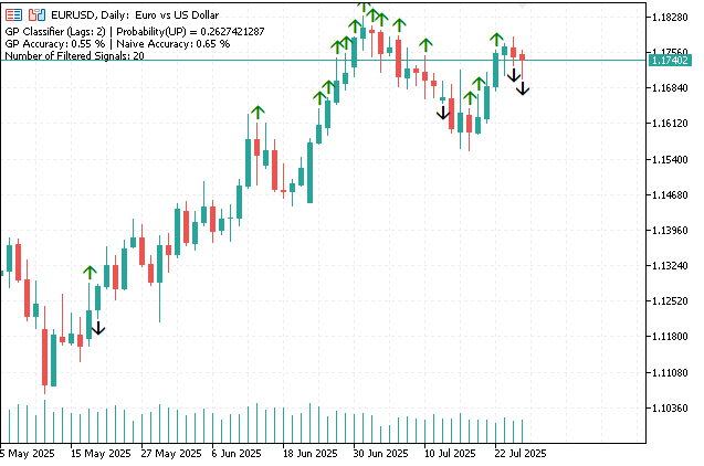
图 4.高斯过程分类器指标(RBF核)的预测结果
计算准确率指标(ShowACCURACY)
启用 ShowACCURACY 参数后,该指标将对最后一个 calculate_bars 执行一次性分类准确率计算,并将 GP 模型预测与“朴素”预测进行比较。
真实标签(y_true)定义为价格变动的实际方向。GP 预测 (gp_pred) - GP 模型预测的标签。“朴素”预测(naive_pred)假设下一个价格走势的方向与前一个走势的方向相同(例如,如果前一根 K 线价格上涨,则朴素预测为增长)。
对两种模型(gp_accuracy 和 naive_accuracy)的 CLASSIFICATION_ACCURACY 指标进行比较,并将结果显示在图表注释中。这使我们能够客观地评估 GP 模型相对于简单基准的性能。
结论
今天,我们已经完成了对高斯过程分类模型的研究。在详细审查了理论结构后,我们能够创建一个基本版本的库,使我们能够解决回归和分类问题。对合成数据的测试证实了所实现的库组件的正确操作,包括有效使用分析梯度和使用高性能的 OpenBLAS 库来提高数值稳定性和速度。
GPRegressor 和 GPClassifier 指标证明了使用 GP 进行实时动态金融时间序列预测的实际可行性,而 RMSE(用于回归)和准确率(用于分类)等指标可以对模型的性能进行客观评估。
然而,该库的实现远非理想。尽管付出了种种努力,但它的速度仍然不如 scikit-learn 等成熟的解决方案。部分原因是由于我们使用的是速度相对较慢的 MinBleic 优化器。
因此,该库的进一步改进可能在以下方面:
- 使用更高效的梯度优化器。特别是,我们需要一种快速的 L-BFGS 算法,对于具有大量超参数的问题,其效率要明显优于当前的算法;
- 更稳健的牛顿法拉普拉斯近似实现。添加线性搜索可以更高效、更可靠地找到后验分布模式,从而提高最终优化的收敛性;
- 稀疏方法的实现。与目前使用全矩阵的工作不同,使用稀疏表示将使库能够在大量数据上进行训练,为扩展和应用 GP 开辟了新的可能性。
本文中用到的程序
| # | 名称 | 类型 | 描述 |
|---|---|---|---|
| 1 | GPClassifier.mq5 | 指标 | 根据预测概率(在线训练)将价格方向提前一步分类 |
| 2 | GPRegressor.mq5 | 指标 | 提前一步预测价格和置信区间(在线训练) |
| 3 | GPsynthetic.mq5 | 脚本 | 在合成数据上测试 GP 模型 |
| 4 | GP.mqh | 类库 | GaussianProcess 类结合了核函数、似然函数和推断方法,而 GPOptimizationObjective 类则负责优化。 |
| 5 | Inference.mqh | 类库 | IInference 接口及其定义推断方法的实现 |
| 6 | Kernels.mqh | 类库 | IKernel 接口和协方差核的实现 |
| 7 | Likelihoods.mqh | 类库 | ILikelihood 接口和似然函数实现 |
| 8 | StructUtils.mqh | 类库 | 辅助函数和数据结构 |
| 9 | DataRegression | CSV | GPsynthetic.mq5 脚本数据 |
| 10 | DataClassification | CSV | GPsynthetic.mq5 脚本数据 |
本文由MetaQuotes Ltd译自俄文
原文地址: https://www.mql5.com/ru/articles/19013
注意: MetaQuotes Ltd.将保留所有关于这些材料的权利。全部或部分复制或者转载这些材料将被禁止。
本文由网站的一位用户撰写,反映了他们的个人观点。MetaQuotes Ltd 不对所提供信息的准确性负责,也不对因使用所述解决方案、策略或建议而产生的任何后果负责。

 交易中的神经网络:时间序列查询模型(结论)
 交易中的神经网络:时间序列查询模型(TQNet)
 新手在交易中的10个基本错误
 运用聪明钱概念(SMC)提升交易水平:订单块(OB)、结构突破(BOS)与公允价值缺口(FVG)

您好,
您好!
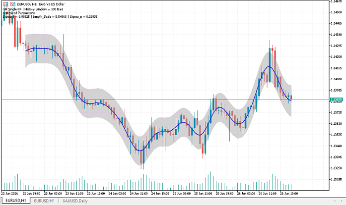
您是想要这样的效果吗?
现在显示的不是下一步的预测,而是训练样本的均值和方差。
非常感谢,您真是太好了。
高斯过程回归模型能否以在线模式进行训练,使其能够实时适应数据的均值和方差?
非常感谢,您真是太贴心了。
能否对基于高斯过程的回归模型进行在线训练,使其能够实时适应数据的均值和方差?