机器学习中的高斯过程（第一部分）：MQL5 中的分类模型

概述

我们将继续了解机器学习模型 — 高斯过程（GP）。在上一篇文章中，我们详细探讨了回归问题，其主要目标是预测连续值。而今天，我们要面对一个更为复杂的话题 — 分类。其难点在于，高斯过程中的分类推断没有封闭形式的解，这需要使用近似方法，如拉普拉斯近似。

为了有效解决这一复杂问题，我们将在 MQL5 中开发一个高斯过程的模块化库。这种方法可以通过将 GP 模型拆分为彼此独立的组件来更好地组织代码，并为进一步的改进和扩展提供坚实的基础。该库将成为回归和分类任务的通用工具。

在本文的第一部分，我们将详细探讨 GP 分类理论，包括近似方法背后的数学原理。同时，我们还将介绍库中的主要类 — GaussianProcess，它将模型的所有组件整合在一起，以及负责与 Alglib 优化库集成的 GPOptimizationObjective 类。

分类

分类是一项机器学习任务，涉及将一个对象分配到预定义的类别中。例如，在金融领域，分类可以根据历史数据帮助预测股票价格是上涨还是下跌。

在本文中，我们将重点讨论二元分类，其中一个对象属于两个类别之一，例如“上升”（+1）或“下降”（-1）。与仅输出类别标签的支持向量机（SVM）或决策树等方法不同，高斯过程允许进行概率预测。例如，一个模型可能会说，一只股票有 75% 的概率会上涨。此类信息在交易中尤其宝贵，因为在交易中，对预测的信心程度有助于做出明智的决策，使人们能够过滤掉不可靠的信号。 

遗憾的是，使用高斯过程解决分类问题比回归问题要复杂得多。这与所使用的似然函数类型有关： 

• 在回归任务中，通常使用高斯似然函数。将高斯过程（作为函数的先验分布）与高斯似然函数相结合，我们可以通过解析方法获得后验分布，从而简化所有计算。
• 对于目标为离散类标签的分类问题，高斯似然并不适用。或者，可以使用例如 logit 似然函数。这导致后验分布也不是高斯分布，也没有闭式解。

因此，我们不得不采用复杂的近似推理方法。这些方法的基本思想是用以众数为中心的高斯分布来近似真实的非高斯后验分布。在本文中，我们将重点介绍拉普拉斯近似，因为它是获得后验分布高斯近似最简单、最有效的方法之一。 

对于二元分类，基于 GP 的预测的基本思想非常简单。我们从潜在函数 f(x) 的先验分布开始。想象一下，GP 生成的不是一个函数，而是一组无穷多的可能函数，其中每一个都是数据中一种可能的隐含依赖关系。然后，这些潜在函数 f(x) 的实现中的每一个都会“通过”逻辑函数（sigmoid）。sigmoid 函数将任何实数（f(x) 的值）转换为 0 到 1 之间的概率，这将是属于 “+1” 类的先验概率 π(x)：

值得注意的是，π 是 f 的确定性函数，但由于 f 本身是随机的（即来自高斯过程的样本），因此函数 π 也变得随机。对于一维输入空间 X，这一概念在图 1 和图 2 中得到了清晰的展示。

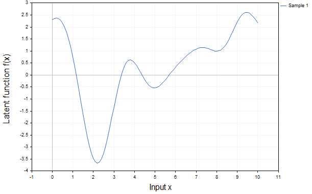
图 1.潜在函数 f(x) 的实现

图 1 仅显示了潜在函数的一种可能实现方式，展示了对应于给定核超参数的函数的典型行为。

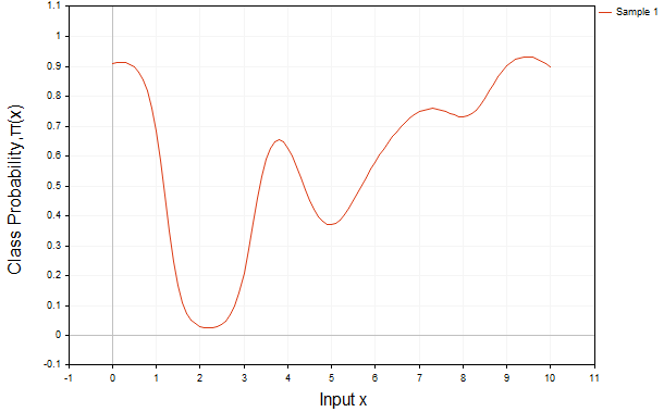
图 2.使用 sigmoid 函数变换后的同一函数

图 2 展示了将逻辑（sigmoid）函数应用于同一函数 f(x) 的结果：

因此，我们得到了类别归属的先验概率分布 π(x)=σ(f(x))，但在这个阶段，该分布尚未考虑训练数据 y。如果没有对 y 的观测，这个先验分布仍只是缺乏经验支持的初始假设；模型也就无法判断哪些先验设想是正确的，哪些需要修正。 

当然，先验假设的选择对最终的后验结果有显著影响。这是贝叶斯方法的一个关键特征，因为函数的先验分布的性质，以及最终模型，取决于研究人员对核类型的决定。 

推理

因此，为了做出有根据的预测，我们需要考虑真实的训练数据 y。这正是进行推断的地方。推理的主要目标是将我们的先验信念转化为后验信念，即根据观察到的数据进行调整后的信念。对于分类问题，这一过程自然分为两个连续的步骤。

步骤 1：潜在函数 f∗ 的预测分布

在第一步中，我们计算给定观测到的训练数据（X, y）时，新测试点 x* 的潜在函数 f* 的后验分布 p(f*|X, y, x*)。该分布由以下积分定义：

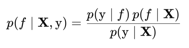
其中：

• p(f*∣X, x*, f) 表示在给定训练点 X 的潜在函数 f 的条件下，新测试点 x* 处的潜在函数 f* 的条件分布。由于高斯过程从定义上讲具有联合正态分布，因此该分布始终为正态分布，
• p(f|X, y) 是训练数据上潜在函数 f 的后验分布。由于似然函数（sigmoid）是非线性的，因此它不是高斯分布。

值得注意的是，由于 p(f|X, y) 并非正态分布，因此该积分没有封闭形式的解。这意味着我们需要采用近似方法来计算它。 

步骤 2：最终预测概率 π*

在第二步中，我们使用这个预测分布来形成最终的概率预测 π* — 即测试点 x* 属于正类（y*=+1）的概率：

这里 σ(f*) 是逻辑（sigmoid）函数，它将潜在函数 f* 的值转换为 0 到 1 之间的概率。积分本身意味着我们根据所有可能的 f* 值对这些概率进行平均，并由它们的后验预测分布进行加权。本质上，这个一维积分是函数 σ(f*) 关于分布 p(f*|X, y, x*) 的数学期望。

同样，对于 logit 似然函数，这个积分也没有封闭形式的解。因此，这里我们也需要使用近似方法。展望未来，我们的 GP 库实现了三种这样的近似方法，使您能够根据精度和计算成本的要求选择合适的方法：

•  Probit 近似
•  数值积分
•  蒙特卡洛方法。

我们刚才描述的这两个步骤 — 计算潜在函数的后验分布，然后进行积分以获得预测概率 — 代表了高斯过程中贝叶斯推断的一般框架。为了获得所需的预测结果，我们需要计算这两个积分，而这两个积分都需要使用近似方法。 

拉普拉斯近似

我们已经了解到，贝叶斯分类推断涉及无法以封闭形式求解的积分。拉普拉斯近似通过用高斯分布 q(f∣X, y) 近似非高斯分布 p(f∣X, y) 来解决这一问题。由于条件分布 p(f*∣X, x*, f) 也是高斯分布，因此得到的预测分布 p(f*∣X, y, x*) 也变为高斯分布。这使我们能够推导出 f* 的均值和方差的分析公式，从而显著简化后续计算。因此，拉普拉斯近似的优点和计算效率在于其能够将后验分布和预测的计算简化为对高斯分布的操作。

重要的是要理解，拉普拉斯近似是一种折衷方案。它使一个原本无法用封闭形式求解的问题在计算上变得可解，但代价是牺牲了准确表示后验分布真实形式的能力。这种正态近似的质量直接取决于 p(f∣X, y) 的真实分布与正态分布的接近程度。二者越接近，近似就越准确，反之亦然。

如果我们关注的是 p(f*∣X, y, x*) 的真实分布，而非其近似值，那么通常会使用马尔可夫链蒙特卡洛（Markov Chain Monte Carlo，MCMC）方法。尽管 MCMC 方法能够提供更准确的估计，但其在计算上成本高昂且难以实施。MCMC 可以作为与近似推理方法进行比较的黄金标准。

现在，让我们仔细了解一下拉普拉斯近似法。这种近似法是围绕真实后验分布 p(f∣X, y) 的众数（最大值）构建的。它使用后验密度对数在该众数附近的二阶泰勒展开式。从数学上讲，我们以下列方式近似后验密度的对数：

其中：

• q(f∣X, y) 是后验分布 p(f∣X, y) 的高斯近似，
• f_hat = argmax(f) p(f|X, y) — 后验分布的众数，
• A = −∇∇ log p(f|X, y)|f=f_hat — 后验分布负对数在众数点处的 Hessian 矩阵。

首先，为了进行拉普拉斯近似，我们需要找到潜在函数f的最可能值，即众数 f_hat。为了获得后验概率 p(f∣X, y)，我们使用贝叶斯规则。我们已经知道，该规则将后验分布与似然函数 p(y∣f)、先验分布 p(f∣X) 以及边际似然函数 p(y∣X) 关联起来，具体如下：

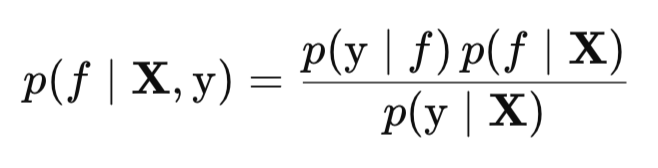
为了使关于 f的p(f∣X, y) 最大化，我们无需知道归一化常数 p(y∣X)，因为它不依赖于 f，因此不会影响最大值的位置。因此，我们可以使用未归一化的后验分布，该分布与似然性和先验分布 p(y∣f)p(f∣X) 的乘积成正比。

为了简化计算并避免在处理非常小的概率值时出现数值问题，我们对这个未归一化的后验分布取对数。由于对数的性质，概率的乘积等于它们对数的和：

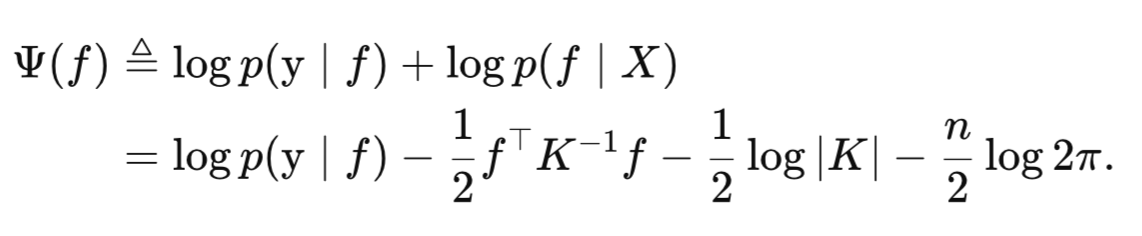
Ψ(f) 是我们将使用牛顿法来最大化的目标函数，以找到潜在函数的极值。牛顿法需要计算 Ψ(f) 对 f 的一阶导数和二阶导数。

将此方程关于 f 求导，我们得到：

其中：

• W = −∇∇ log p(y|f) - 对数似然函数的负 Hessian 矩阵，这是一个对角矩阵。

计算出梯度和 Hessian 矩阵后，我们使用牛顿法迭代地寻找众数：

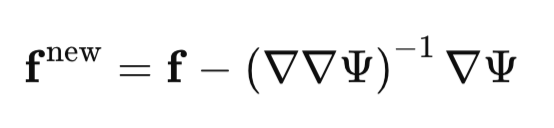
在每次迭代中，牛顿法都会根据梯度和 Hessian 矩阵确定的方向更新我们当前对众数的估计，直到达到收敛为止。 

一旦确定了众数，我们就可以计算近似高斯分布的协方差矩阵。该矩阵等于在众数点 (f{hat}) 处计算得到的 Hessian 的负逆矩阵。

因此，我们高斯近似的协方差矩阵 Σ 为：

至此，拉普拉斯近似的第一步 — 寻找后验分布的正态近似 — 的描述已告完成。

拉普拉斯近似中的预测

一旦我们获得了 q(f∣X, y)，就可以进行推理的第二步 — 对新测试点 x∗ 进行预测。在这一阶段，我们要找到预测分布 p(f∗∣X, y, x∗)。由于拉普拉斯近似使 p(f∣X, y) 变为高斯分布（形式为 q(f∣X, y)），并且 p(f∗∣X, x∗, f) 也是高斯分布，因此得到的预测分布 p(f∗∣X, y, x∗) 也变为高斯分布。这使我们能够通过解析方式获得其后验均值和方差。

对于新的测试点 x*，潜在函数 f* 的均值 (mu_f_star) 计算如下：

对于新的测试点 x*，潜在函数 Var(f*) 的方差（Sigma_f_star）计算如下：

现在我们有了预测分布的均值和方差，我们终于可以计算所需的类别归属概率 π* 了： 

这个公式是基于拉普拉斯的 GP 分类器中概率预测的核心。

你可能已经注意到，我们并不是简单地将类概率计算为 σ(E[f∗])，即直接将 f∗ 的后验均值代入 sigmoid 函数。这种方法被称为 MAP 预测（最大后验概率预测），它当然有存在的理由。

然而，在计算最大后验概率（MAP）预测 σ(E[f∗]) 时，我们忽略了 f* 的不确定性。我们只是简单地取中心估计 f*（即均值），并将其转换为概率。在计算 E[σ(f*)]（对应于积分）时，我们考虑了 f* 分布的整体形状。这为我们提供了更准确、更有意义的预测概率，尤其是在 f* 存在显著不确定性（即 V[f*] 的方差较大）或 f* 的分布不对称时。这种方法称为平均预测概率。

理解这种差异具有重要的实际意义：

• 如果你的唯一目标是获得一个二元类别标签（例如，“买入”或“卖出”，+1 或 -1），那么使用更简单的最大后验概率预测可能就足够了，因为它会得出与计算成本更高的平均预测相同的标签。
• 然而，如果你更关心概率本身，那么平均预测概率（E[σ(f*)]）仍然更为准确，因为它们充分考虑了模型的不确定性。 

在交易中，仅凭简单的二元分类标签（“买入”或“卖出”）是远远不够的。我们需要概率所带来的更细粒度的置信水平。概率值使我们能够过滤交易信号。一个成功概率为 0.51（仅略高于随机猜测）的信号，其价值远低于成功概率为 0.60 的信号。这使得交易者能够设定进入交易的阈值。例如，我们可以决定，只有当成功概率高于 0.55 或 0.60 时，才会开立交易，从而减少错误信号的数量。

拉普拉斯近似中的边际似然

既然我们已经了解了高斯过程在分类中的推理机制，那么问题就来了：如何调整我们的模型以获得最佳预测？答案在于边际似然（LML）。这是我们用来优化模型超参数 θ 的目标函数。如果不计算它，就无法找到解释我们数据的最佳参数： 

其中，B

在定义了待优化的目标函数后，下一个重要步骤是计算其关于超参数 θ 的偏导数。这是必要的，因为我们将使用解析梯度进行优化。与数值方法相比，这种方法可以提高计算速度数倍。解析梯度使优化器能够更高效、更准确地向 NLML 目标函数的最小值移动。 

LML 梯度由显式部分和隐式部分组成：

计算显式部分的公式：

这里的主要问题是计算核矩阵 K 关于每个超参数的导数。我们将在本文的第二部分讨论所选核函数的导数实现。

隐式部分由两个因子构成。隐式部分中的第一个因子可以用以下公式求得：

要计算这个公式，我们需要计算似然函数对数的三阶导数。

隐式部分的第二个乘数计算如下： 

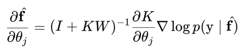
总之，我们注意到，NLML 不仅用于估计超参数，还用于比较不同的模型（例如，使用不同类型的核函数）。具有较低 NLML 值的模型被认为更好，因为这意味着边际似然更高，即模型对观测数据的解释能力更强。

此外，高斯过程通过使用边际似然来优化超参数，从而自动解决了数据拟合与模型复杂度之间的权衡问题。NLML 自然会惩罚过于复杂的模型，从而防止过拟合。因此，无需像训练神经网络时那样，设置明确的停止标准来防止过拟合。NLML 优化本身力求找到最佳平衡点。这是贝叶斯方法应用于高斯过程的主要优势之一。

高斯过程库

既然我们已经涵盖了所有必要的理论概念，接下来就让我们转向实际实现。我们的主要目标是在 MQL5 中创建一个通用的 GP 库，作为预测任务的可靠工具。该库将采用模块化架构，其中 GP 模型被分解为独立、可互换的组件，这将便于扩展其功能并确保易于维护。在开发过程中，我们将考虑以下关键功能特性：

• 核函数选择灵活性：能够轻松连接现有的协方差核函数，以及创建它们的组合（如SumKernel、ProductKernel）以建模更复杂的依赖关系；
• 支持多种似然函数；
• 支持用于分类和回归问题的各种后验分布推断方法；
• 多功能性：库必须具备通用性，能够同时解决回归和二分类问题；
• 超参数优化：利用解析梯度来提高训练过程的速度和准确性。与 Alglib 库的集成应能确保模型超参数的高效优化。

让我们仔细看看库的结构。它由六个主要组件组成，每个组件都实现了特定的功能：

• GaussianProcess 类是该库的核心，管理着 GP 模型的整个生命周期 — 从初始化和超参数优化到对新数据进行预测。

• GPOptimizationObjective 类：这个辅助类充当我们库和 Alglib 优化库之间的“桥梁”。它将目标函数及其梯度调整为 Alglib 所需的格式（通过继承 CNDimensional_Grad）。

• IKernel 接口：定义了一系列用于各种协方差函数（核函数）的方法。它包括 RBFKernel、LinearKernel、PeriodicKernel 等实现，以及它们的组合（SumKernel、ProductKernel）。

• ILikelihood 接口：定义了一组似然函数方法。实现方式包括用于回归的 GaussianLikelihood 和用于二元分类的 LogitLikelihood。

• IInference 接口：提供用于推断潜在高斯过程函数后验分布的方法。目前，已实现了 ExactInference 和 LaplaceInference。

• 辅助结构和公用设施（StructUtils.mqh）：一组常用的枚举、数据结构（用于推理和预测结果）以及处理数据、矩阵和图表以可视化结果所需的函数。

由于采用了模块化结构和定义良好的接口，我们可以轻松添加新的核函数ß、推理方法和似然函数，从而方便库的未来发展。 

GaussianProcess 类

GaussianProcess 类是该库的核心类。它包含了构建、训练和预测 GP 模型所需的所有逻辑。GaussianProcess 是按照组合原则设计的，它不直接包含核函数、似然函数或推理功能。它不是通过这种方式，而是通过三个主要接口来集成这些组件：

• 核函数（IKernel），
• 似然函数（ILikelihood），
• 推理方法（IInference）。

这样一来，GP 模型就可以灵活地适应各种预测任务，而无需改变底层的 GaussianProcess 类。

//+------------------------------------------------------------------+
//| Gaussian process class                                           |
//+------------------------------------------------------------------+
class GaussianProcess
{
private:
    IKernel*      m_kernel;       // pointer to the selected kernel
    ILikelihood*  m_likelihood;   // pointer to the selected likelihood function
    IInference*   m_inference;    // pointer to the selected inference method
    matrix        m_X_train;      // Training input data Nxd
    vector        m_y_train;      // Training target data Nx1

    GPInferenceResult m_last_inference_result; // Structure storing the latest inference results
    
    int m_last_termination_type;  // Optimization operation completion code
    int m_last_iterations_count;  // Number of iterations performed by the optimizer
    double m_last_nlml_value;     // Final NLML value after optimization
    
private:
    // Auxiliary function for numerical integration
    double CalculateNumericalProbability(double mu_f_star, double sigma_f_star_diag, LogitLikelihood *likelihood);

public:
    // Class constructor
    GaussianProcess(IKernel* kernel, ILikelihood* likelihood, IInference* inference,
    const matrix &X_train, const vector &y_train);
    // Static method for creating a GaussianProcess object with input parameters validation
    static GaussianProcess* Create(IKernel* kernel, ILikelihood* likelihood, IInference* inference,
    const matrix &X_train, const vector &y_train);
    
    // Destructor
    ~GaussianProcess();
    
    // --- Methods for getting the model state ---
    // Return the results of the last inference operation
    GPInferenceResult GetLastInferenceResult() const;
    // Return the completion type of the last hyperparameter optimization
    int GetLastTerminationType() const;
    // Return the number of iterations performed during the last hyperparameter optimization
    int GetLastIterationsCount() const;
    // Return the negative logarithm of the marginal likelihood after optimization
    double GetLastNLML() const;
    // Return the pointer to the kernel in use
    IKernel* GetKernel() const;
    // Return the current values of all hyperparameters being optimized.
    vector GetCurrentHyperparameters();
  
    // --- Training and configuration methods ---
    // Run the full model training process, including hyperparameter optimization
    bool Fit();
    // Perform a single inference step without hyperparameter optimization
    bool PerformInference();
    // Set the training data for the model 
    void SetTrainingData(const matrix& X, const vector& y);
    // Set the given hyperparameters for the kernel and likelihood function
    void SetHyperparameters(const vector &params);
    // Method called by the optimizer to calculate the objective function (NLML)
    double CalculateNLMLObjective(const vector &hyperparameters);
    
    // --- The method performs a prediction for new test data
    // The predictmode parameter determines the method for calculating probabilities for classification (PROBIT, NUM_INTEGR, MONTE_CARLO)
    bool Predict(const matrix &X_test, GPPredictionResult &result, PredictMode mode = PROBIT);
    
    // --- Auxiliary methods ---
    // Static method for generating samples from prior GP
    static bool SamplePriorGP(const matrix &x, IKernel* kernel, int num_samples, matrix &f_samples,
                              bool plot_samples = false, int plot_display_seconds = 10);
    //--- Method for logging the final values of hyperparameters
    void PrintOptimizedKernelParameters();  
}; 

让我们来看一下这个类的主要方法：

创建类实例主要有两种方法：

• Create 方法：使用此方法可以安全地创建 GaussianProcess 对象。此方法对输入数据（X_train、y_train、接口指针）执行必要的检查，并在出错时返回指向对象的指针或 NULL。

//+------------------------------------------------------------------+
//| Create method                                                    |
//+------------------------------------------------------------------+
GaussianProcess* GaussianProcess::Create(IKernel* kernel, ILikelihood* likelihood, IInference* inference,
const matrix &X_train, const vector &y_train)
{
    // 1. Check for NULL pointers
    if (kernel == NULL || likelihood == NULL || inference == NULL) {
        Print("ERROR: Kernel, Likelihood, or Inference pointer is NULL");
        return NULL;
    } 
    // 2. Check the validity of X_train and y_train inputs
    if (X_train.Rows() == 0 || y_train.Size() == 0 || X_train.Rows() != y_train.Size()) {
    Print("ERROR: Invalid training data dimensions");
    return NULL;
    }
    // 3. Check the compatibility of 'likelihood' and 'inference'
    string likelihood_name = likelihood.GetName();
    string inference_name  = inference.GetName();   
    if (inference_name == "ExactInference" && likelihood_name != "GaussianLikelihood") {
        Print("ERROR: ExactInference supports only GaussianLikelihood!");
        delete kernel; delete likelihood; delete inference;
        return NULL;
    }    
    // 4. If all checks are passed, create the object
    GaussianProcess* gp_model = new GaussianProcess(kernel, likelihood, inference,X_train, y_train);
    if (gp_model == NULL) {
        Print("ERROR: Failed to create GaussianProcess object");
        delete kernel; delete likelihood; delete inference;
        return NULL;
    }    
    return gp_model;
} 

• 类构造函数：提供了一种直接的初始化方法，无需任何数据检查。如果您对自己的数据有信心，可以使用构造函数创建一个对象。

//+------------------------------------------------------------------+
//| GaussianProcess class constructor                                |
//+------------------------------------------------------------------+
GaussianProcess::GaussianProcess(IKernel* kernel, ILikelihood* likelihood, IInference* inference,
const matrix &X_train, const vector &y_train) :
    m_kernel(kernel),
    m_likelihood(likelihood),
    m_inference(inference),
    m_X_train(X_train), 
    m_y_train(y_train), 
    m_last_termination_type(0),
    m_last_iterations_count(0),
    m_last_nlml_value(0.0){ } 

• Fit() 方法：启动完整的模型训练过程。该方法使用 MinBleic 优化器来优化核超参数和似然函数，该优化器能够最小化负对数边际似然（NLML）。

//+------------------------------------------------------------------+
//| Method for training the model                                    |
//+------------------------------------------------------------------+
bool GaussianProcess::Fit()
{
    // Create the GPOptimizationObjective object passing it the pointer to the current GaussianProcess object
    // This pointer goes into the private field of the m_gp class, with which we call the method
    // CalculateNLMLObjective to get the NLML value for the current set of hyperparameters
    GPOptimizationObjective objective_func(GetPointer(this));
    CNDimensional_Rep frep; 
    CObject Obj;
    vector initial_hyperparams = GetCurrentHyperparameters(); // Get the initial values of the hyperparameters
    double theta[];
    ArrayResize(theta, (int)initial_hyperparams.Size()); 
    VectorToArray(initial_hyperparams,theta);
    int num_params = (int)initial_hyperparams.Size();
    double s[];
    double bndl[];
    double bndu[];
    ArrayResize(s, num_params);
    ArrayResize(bndl, num_params);
    ArrayResize(bndu, num_params);

    int param_idx = 0; 
    IKernel* kernels_to_process[]; // array of pointers to the IKernel interface
    
    // Logic for obtaining kernels to set boundaries 
    // This block of code determines what type of kernel we are dealing with
    // and fills the kernels_to_process array with the corresponding pointers:
    if (dynamic_cast<SumKernel*>(m_kernel) != NULL) {          // Check if the current kernel m_kernel is a SumKernel object  
        SumKernel* sum_k = dynamic_cast<SumKernel*>(m_kernel); // If yes, then we cast the m_kernel type to the SumKernel* type
        sum_k.GetKernels(kernels_to_process); // and call the GetKernels() method, which fills the kernels_to_process array with all the kernels included in the sum
    } else if (dynamic_cast<ProductKernel*>(m_kernel) != NULL) { // Similar logic if the kernel is a ProductKernel object
        ProductKernel* prod_k = dynamic_cast<ProductKernel*>(m_kernel);
        prod_k.GetKernels(kernels_to_process);
    } else {
        ArrayResize(kernels_to_process,1); // If the kernel is neither a sum nor a product (i.e. it is not a composite kernel), 
        kernels_to_process[0] = m_kernel; // then the kernels_to_process array simply contains a pointer to m_kernel.
    }

   // This loop iterates over each base kernel found in the kernels_to_process array
   // and sets its hyperparameters to an initial scale s, a lower bound bndl, and an upper bound bndl
    for(int i = 0; i < ArraySize(kernels_to_process); i++) {
        IKernel* current_k = kernels_to_process[i];
            string kernel_name = current_k.GetName();   
            if (kernel_name == "RBFKernel") {
                if (param_idx + 2 <= num_params) {    
                    s[param_idx] = 1.0; bndl[param_idx] = 1e-3; bndu[param_idx] = 1e3; param_idx++;    
                    s[param_idx] = 1.0; bndl[param_idx] = 1e-3; bndu[param_idx] = 1e3; param_idx++;    
                } 
            } else if (kernel_name == "LinearKernel") {
                if (param_idx + 1 <= num_params) {
                    s[param_idx] = 1.0; bndl[param_idx] = 1e-3; bndu[param_idx] = 1e3; param_idx++;    
                } 
            } else if (kernel_name == "PeriodicKernel") {
                if (param_idx + 3 <= num_params) {
                    s[param_idx] = 1.0; bndl[param_idx] = 1e-3; bndu[param_idx] = 1e3; param_idx++;    
                    s[param_idx] = 1.0; bndl[param_idx] = 1e-3; bndu[param_idx] = 1e3; param_idx++;    
                    s[param_idx] = 1.0; bndl[param_idx] = 1e-3; bndu[param_idx] = 1e3; param_idx++;    
                } 
            }           
    }
    
// --- Add bounds and scales for likelihood parameters (if any) ---
// LogitLikelihood has no hyperparameters, so this block will be skipped for it
// GaussianLikelihood has 1 parameter (sigma)
if (m_likelihood.GetNumHyperparameters() > 0) {
    if (param_idx + m_likelihood.GetNumHyperparameters() <= num_params) {
        s[param_idx] = 1.0;           // Scale
        bndl[param_idx] = 1e-10;      // Lower bound 
        bndu[param_idx] = 1e3;        // Upper bound
        param_idx++;
    } 
}
    CMinBLEICStateShell state;
    CMinBLEICReportShell rep; // object that will contain a report on the optimization results
    //-----------------------  optimizer stopping criteria
    double epsg = 0.0001;     //Gradient precision (0 means gradient stopping is disabled)
    double epsf = 0.0000;     //Precision by function value    
    double epsw = 0.0000;     //Accuracy by parameters 
    //-------------------------   
    double epso = 0.00001;    //Parameters for external convergence conditions in BLEIC
    double epsi = 0.00001;    //Parameters for internal convergence conditions in BLEIC
    CAlglib::MinBLEICCreate(theta, state);       // initialize the optimizer. It creates the initial state for MinBLEIC using the initial hyperparameter values from the theta array.
    CAlglib::MinBLEICSetBC(state, bndl, bndu);   // Set the lower (bndl) and upper (bndu) bounds for each parameter
    CAlglib::MinBLEICSetScale(state, s);         //Sets the scales (s) for each parameter. This can help the optimizer work more efficiently with parameters of different orders of magnitude.
    CAlglib::MinBLEICSetInnerCond(state,epsg,epsf,epsw);    
    CAlglib::MinBLEICSetOuterCond(state, epso, epsi);    
    CAlglib::MinBLEICOptimize(state, objective_func, frep, 0, Obj); // start the optimization    
    CAlglib::MinBLEICResults(state, theta, rep); // optimization report
    
    m_last_termination_type = rep.GetTerminationType();
    m_last_iterations_count = rep.GetInnerIterationsCount();
    m_last_nlml_value = objective_func.GetNLML(); // Get the final NLML
//------------------------------------------------------------------------------------    
//    TerminationType field contains completion code, which can be:
//-8     internal integrity control detected    infinite    or    NAN    values    in
//     function/gradient. Abnormal termination signalled.
//-3     inconsistent constraints. Feasible point is
//     either nonexistent or too hard to find. Try to
//     restart optimizer with better initial approximation
// 1     relative function improvement is no more than EpsF.
// 2     relative step is no more than EpsX.
// 4     gradient norm is no more than EpsG
// 5     MaxIts steps was taken
// 7     stopping conditions are too stringent,
//     further improvement is impossible,
//     X contains best point found so far.
// 8     terminated by user who called minbleicrequesttermination(). X contains
//     point which was "current accepted" when    termination    request    was
//     submitted.
//-------------------------------------------------------------------------------------  
// Determine the success of optimization based on TerminationType
    bool success = true;     
    if (m_last_termination_type < 0)
    {
        Print("Error: GP optimization failed. Completion type: ", m_last_termination_type);
        success = false;
    } 
    // Update the model hyperparameters after optimization
    vector optimized_hyperparams;
    optimized_hyperparams.Assign(theta);
    SetHyperparameters(optimized_hyperparams);   
    return success;     
} 

在 Fit() 方法内部，我们准备了优化器有效工作所需的一切。

创建了一个特殊对象 objective_func (GPOptimizationObjective)，它以 Alglib 可理解的格式表示 NLML 目标函数及其解析梯度。将指向当前 GaussianProcess 对象的指针传递给其构造函数（这是调用 CalculateNLMLObjective 方法所必需的）。

接下来，我们获取 theta 超参数数组中所有模型超参数的当前值。这些值（从核函数和似然函数中获得）将作为寻找最优值的起点。对于每个超参数，都指定了尺度（s）、下限（bndl）和上限（bndu）。这些边界可以防止在不适定或无意义的区域（例如，负的尺度长度或方差）中搜索解。优化器使用缩放比例来归一化参数，这可以提高稳定性和收敛速度，尤其是在参数数量级差异较大时。默认值 s = 1.0

接下来，我们声明一个指向 Ikernel 接口的 kernels_to_process 指针数组。它将用于存储所有需要优化超参数的基础核函数列表。如果我们有一个简单的核函数（不是复合核函数），那么这个数组将只有一个元素 — 指向该核函数的指针。如果是 SumKernel 或 ProductKernel，则它将存储指向构成此组合的所有核函数的指针。

接下来，使用 dynamic_cast 运算符，我们检查当前核函数 m_kernel（它是 GaussianProcess 类的一个字段，指向用户选择的核函数）是否是 SumKernel 或 ProductKernel 的实例。如果是这样，则会进行类型转换，转换为 SumKernel 或 ProductKernel，并调用 GetKernels() 方法，该方法会将包含在核函数和或核函数积中的所有核函数填充到 kernels_to_process 数组中。如果核函数既不是求和也不是乘积（即它是一个常规核函数，如 RBF 核函数），则 kernels_to_process 数组仅包含一个指向 m_kernel 本身的指针。

之后，我们遍历 kernels_to_process 中找到的每个基本核函数，并将其超参数设置为缩放 s 并限制 bndl 和 bndu。

最后，在处理完所有核函数超参数之后，再处理似然函数超参数。高斯似然函数有一个参数，而逻辑似然函数没有参数。所有参数准备就绪后，优化过程开始。

• CalculateNLMLObjective() 方法充当主 GaussianProcess 类和外部 Alglib 优化器之间的链接。这正是 MinBleic 优化器不断调用（通过 GPOptimizationObjective 类）来评估当前超参数值的目标函数。它的主要任务是返回给定超参数集的 NLML 值。

//+-------------------------------------------------------------------+
//| Method that will be called by the optimizer to calculate NLML     |
//+-------------------------------------------------------------------+
double GaussianProcess::CalculateNLMLObjective(const vector &hyperparameters)
{
    //  Set all hyperparameters (kernels and likelihoods)
    SetHyperparameters(hyperparameters);    
    //  Call the inference function, which will calculate NLML
    m_inference.Infer(m_X_train, m_y_train, m_kernel, m_likelihood,m_last_inference_result);
    if (!m_last_inference_result.success) {    
        Print("Inference Error !");
        return DBL_MAX;    
    }    
    return m_last_inference_result.nlml_value;
}

在每次迭代中，MinBleic 优化器都会提出一组新的超参数。CalculateNLMLObjective() 函数首先会获取这组超参数，并使用 SetHyperparameters() 方法来更新核函数（m_kernel）和似然函数（m_likelihood）对象中的相应参数。这非常重要，因为所有后续的 NLML 计算都应该基于这些当前的超参数值。

更新超参数后，该方法对推理对象 (m_inference) 调用 Infer()。这是进行所有旨在估计后验分布的复杂数学计算的主要步骤。

推理结果（包括 NLML 值及其梯度，这些将被 Grad 函数使用）存储在私有类字段 m_last_inference_result 中。

如果推理成功，该方法返回 NLML。

• GaussianProcess::SetHyperparameters(const vector &params) 方法负责分发和设置核超参数和似然函数的优化值。 

//+------------------------------------------------------------------+    
//| Method for setting hyperparameters                               |
//+------------------------------------------------------------------+
void GaussianProcess::SetHyperparameters(const vector &params)
{
//+------------------------------------------------------------------+    
//This is a call of the polymorphic SetHyperparameters method on the object pointed to by m_kernel.
//Since m_kernel is a pointer to a base type (IKernel*), calling SetHyperparameters
//will be redirected to a concrete implementation of this method in the derived kernel class
//m_kernel refers to. For example, if m_kernel actually points to an object
//RBFKernel, RBFKernel::SetHyperparameters(params) is called. If this is SumKernel, 
//the SumKernel::SetHyperparameters(params) method is called, and so on.    
//+------------------------------------------------------------------+
    int kernel_params_count = m_kernel.GetNumHyperparameters();
    int likelihood_params_count = m_likelihood.GetNumHyperparameters();
    // Set kernel parameters
    vector kernel_hps(kernel_params_count);
    for(int i = 0; i < kernel_params_count; i++) {
        kernel_hps[i] = params[i];
    }
    m_kernel.SetHyperparameters(kernel_hps);    
    // Set the likelihood parameters
    vector likelihood_hps(likelihood_params_count);
    for(int i = 0; i < likelihood_params_count; i++) {
        likelihood_hps[i] = params[kernel_params_count + i];
    }
    m_likelihood.SetHyperparameters(likelihood_hps);
}

params 向量按固定顺序包含高斯过程模型的所有超参数：首先是核函数（如果是复合核函数，则为多个核函数）的所有超参数，然后是似然函数的参数。该方法的关键特点是利用了多态性。对 m_kernel.SetHyperparameters() 的相同调用，根据运行时 m_kernel 指向的对象的实际类型而表现不同。 

• Predict() 方法。这基本上就是构建模型的目的：基于新数据进行预测。 

//+------------------------------------------------------------------+
//| Prediction method for regression and classification              |
//+------------------------------------------------------------------+    
bool GaussianProcess::Predict(const matrix &X_test, GPPredictionResult &result,PredictMode predict_mode)
{     
    // 1. Check that the model has been trained
    if (!m_last_inference_result.success) {
        Print("Error: Predict - Inference results not available");
        return false;
    }
    // 1.1 Check the match of the number of features
    if (X_test.Cols() != m_X_train.Cols()) {
        Print("Error: Predict - Number of features in X_test  must match X_train ");
        return false;
    }

    int N_train = (int)m_X_train.Rows();
    int N_test = (int)X_test.Rows();

    // 2. K_s and K_ss are calculated regardless of the type of inference/likelihood
    matrix K_s = m_kernel.Compute(m_X_train, X_test);            
    matrix K_ss = m_kernel.Compute(X_test, X_test);
    
    // --- 3. Logic for calculating mu_f_star and Sigma_f_star (common for both types of problems) ---
    //------------------------- Algorithm 2.1 GPML----------------------------------------
    if (m_inference.GetName() == "ExactInference") {
        // For ExactInference
        matrix L_K_noisy = m_last_inference_result.L_K_noisy;
        vector alpha = m_last_inference_result.alpha;
        
        result.mu_f_star = K_s.Transpose() @ alpha;            

        matrix V(N_train, N_test);    
        if (!L_K_noisy.LinearEquationsSolution(K_s, V)) {
            Print("Error: Predict (Exact) - LinearEquationsSolution failed");
            return false;        
        }          
        result.Sigma_f_star = K_ss - V.Transpose() @ V;

    } else if (m_inference.GetName() == "LaplaceInference") {
    //------------------------- Algorithm 3.2 GPML ----------------------------------------
        matrix W = -1 * m_last_inference_result.H;    
        matrix L_B = m_last_inference_result.L_B;    
        matrix sW = m_last_inference_result.sW;        
        vector f_hat = m_last_inference_result.mu_f_train;    
        vector grad_f_hat = m_likelihood.LogLikelihoodGradient(f_hat, m_y_train);
        // Eq[f*∣X,y,x*]=k(x*)^T K^−1 f_hat = k(x*)^T ∇log p(y∣f_hat) 
        result.mu_f_star = K_s.Transpose() @ grad_f_hat;
        
        matrix SwKs = sW @ K_s;
        matrix V(N_train, N_test);    
        if (!L_B.LinearEquationsSolution(SwKs, V)) {
            Print("Error: Predict (Laplace) - LinearEquationsSolution failed");
            return false;
        }
        // Vq[f*|X, y,x*] = Kss - Ks^T(K + W^-1)^-1 Ks
        result.Sigma_f_star = K_ss - V.Transpose() @ V;
    }    
    
    // --- 4. Likelihood-specific logic (Likelihood) ---
if (m_likelihood.GetName() == "GaussianLikelihood") {
    // --- 4.1. Regression (GaussianLikelihood) ---
    double noise_variance = 0.0;
    vector likelihood_params = m_likelihood.GetHyperparameters();
    if (likelihood_params.Size() > 0) {
        noise_variance = likelihood_params[0] * likelihood_params[0];
    }    
    result.Sigma_y_star = result.Sigma_f_star + matrix::Identity(N_test, N_test) * noise_variance;
    result.mu_y_star = result.mu_f_star; // For Gaussian likelihood mu_y_star = mu_f_star

    } else if (m_likelihood.GetName() == "LogitLikelihood") {
        // --- 4.2. Classification (LogitLikelihood) ---
          // Make sure m_likelihood is a LogitLikelihood to access the sigmoid method
        LogitLikelihood *logit = dynamic_cast<LogitLikelihood*>(m_likelihood);
        if (logit == NULL) {
            Print("Error: Failed to cast m_likelihood to LogitLikelihood in Predict");
            return false;
        }
        
        result.predicted_probabilities.Resize(N_test);
        result.predicted_labels.Resize(N_test);
        double mc_samples_array[]; 
 
        for (int i = 0; i < N_test; i++) {
            double mu_f_star_i = result.mu_f_star[i];  //mean of the posterior distribution q(f*|X,y,x*)
            double sigma_f_star_diag_i = result.Sigma_f_star[i, i]; // variance of the posterior distribution q(f*|X,y,x*)
    //------------------- 1)Probit Approximation----------------------
            if (predict_mode == PROBIT) {
                double k_i = 1.0 / MathSqrt(1.0 + M_PI / 8.0 * sigma_f_star_diag_i);
                result.predicted_probabilities[i] = logit.sigmoid(mu_f_star_i * k_i);}
    // ----------------- 2) Numerical integration ---------------------------------------
            else if (predict_mode == NUM_INTEGR) {  
                result.predicted_probabilities[i] = CalculateNumericalProbability(
                    mu_f_star_i,
                    sigma_f_star_diag_i,
                    logit
                );} 
   // ----------------------3) Monte Carlo Method ---------------------------------------              
            else if (predict_mode == MONTE_CARLO) {      
                // Number of samples for Monte Carlo
                int num_samples = 10000;                
                ArrayResize(mc_samples_array, num_samples); 
                double std_dev_f_star_i = MathSqrt(sigma_f_star_diag_i);
                // Generate num_samples values from N(mu_f_star_i, std_dev_f_star_i)             
                MathRandomNormal(mu_f_star_i, std_dev_f_star_i, num_samples, mc_samples_array);
                double sum_sigmoid_samples = 0.0;
                for (int s = 0; s < num_samples; s++) {
                    sum_sigmoid_samples += logit.sigmoid(mc_samples_array[s]);
                }
            //To get the expected probability p(y*=+1|X,y,x*)
            //we calculate the arithmetic mean of all obtained values σ(f_sample*). 
            //By the law of large numbers, when num_samples is large enough, 
            //this average will be a good approximation of the true value of the integral     
                result.predicted_probabilities[i] = sum_sigmoid_samples / num_samples;
            }    
            // Predicted labels (+1 or -1)
            result.predicted_labels[i] = (result.predicted_probabilities[i] >= 0.5) ? 1.0 : -1.0;
        }
    }
    return true;    
    }

预测结果（均值、方差、概率、类别标签）被设置为 GPPredictionResult 结构。

首先，我们计算矩阵 K* 和 K**。这些矩阵是高斯过程预测的基础。需要它们来计算潜在函数 f* 在新测试点的均值和方差。这里的逻辑取决于训练过程中使用了哪种推理方法（精确推理（ExactInference）或拉普拉斯推理（LaplaceInference）），因为它们为预测公式提供了不同的组成部分（Rasmussen 和 Williams 所著《GPML》一书中，精确推理对应算法2.1，拉普拉斯推理对应算法3.2）。

如果使用 ExactInference，则会检索预先计算的 L_K_noisy 和 alpha。如果使用 LaplaceInference，则提取 W、L_B、sW 和 f_hat（众数）。在这两种情况下，结果都是每个测试点的潜在函数的均值（mu_f_star）和协方差矩阵（Sigma_f_star）。

正如我们在文章的理论部分已经讨论过的，在计算积分以获得类别概率时存在一个问题。因此，需要使用近似值：

• predict_mode == PROBIT（Probit 近似）：

这是一个常用的快速近似方法。它用形状相似的正态分布的累积分布函数代替了 sigmoid 函数。这使我们能够通过解析方法计算积分。

• predict_mode == NUM_INTEGR（数值积分）：

在此模式下，将调用 CalculateNumericalProbability 辅助函数。它通过将 f* 的范围划分为离散区间并对区间值求和，来数值近似计算积分。它可能更准确，但速度较慢。 

• predict_mode == MONTE_CARLO（蒙特卡洛方法）：

这是一种随机方法。从后验分布 q(f*∣X, y, x*) 生成大量随机样本 f*。对于每个样本 f*，计算 sigma(f*)。

所有这些值的算术平均值 sigma(f*) 是所需概率 p(y*=+1|X, y, x*) 的近似值。这是计算成本最高的方法。为了从正态分布中生成样本，我们使用了 MathRandomNormal 标准库函数。

根据计算出的概率，对上述每种近似方法的预测类别标签做出决策。如果属于 +1 类的概率大于或等于 0.5，则预测为 +1，否则为 -1。

GPOptimizationObjective 类

//+------------------------------------------------------------------+
//| Class for the Alglib optimizer objective function                |
//+------------------------------------------------------------------+
class GPOptimizationObjective : public CNDimensional_Grad
{
private:  
    GaussianProcess* m_gp; // pointer to GaussianProcess object
    double nlml;           // Negative log-likelihood
public:
    // Constructor 
    GPOptimizationObjective(GaussianProcess* gp_instance) : m_gp(gp_instance), nlml(0.0) {}
    double GetNLML() { return nlml; }
    ~GPOptimizationObjective() {}

    // Grad method that will be called by the optimizer
    virtual void Grad(CRowDouble &w, double &func,CRowDouble &grad, CObject &obj) override {     
        // Convert CRowDouble to a vector for passing to GP
        vector hyperparameters(w.Size());
        for(int i = 0; i < (int)w.Size(); i++) { 
           hyperparameters[i] = w[i];        
        }
        
        // Call the GP method to calculate NLML
        func = m_gp.CalculateNLMLObjective(hyperparameters);
        nlml = func; 
        
         GPInferenceResult current_result = m_gp.GetLastInferenceResult(); 
        if (!current_result.success ) {
            Print("Warning: GPOptimizationObjective::Grad - Gradient calculation failed");
            for(int i = 0; i < (int)w.Size(); i++) {
                grad.Set(i, DBL_MAX); 
            }
            return;
        }            
        // Fill grad with elements from current_result.nlml_gradient
        for(int i = 0; i < (int)w.Size(); i++) {
        grad.Set(i, current_result.nlml_gradient[i]);
        }       
    }      
};

该类是我们的 GaussianProcess 类与外部 Alglib 优化库（具体来说是 MinBLEIC 优化器）之间的连接。

Alglib 要求其优化的目标函数必须符合特定的接口。这正是 GPOptimizationObjective 的用途。它继承自定义此接口的 Alglib 基类 CNDimensional_Grad。该基类提供了 GPOptimizationObjective 类应该实现的虚方法。这些方法使得 Alglib 优化器能够处理任何目标函数，只要该函数能同时提供函数值及其梯度。 

私有成员 GaussianProcess* m_gp 包含指向我们的 GaussianProcess 对象的指针。这样，GPOptimizationObjective 类就可以调用 CalculateNLMLObjective 方法来执行必要的计算。 

Grad() 方法是该类中最重要的部分。它重写了 CNDimensional_Grad 中的虚方法，并在每次迭代中由 Alglib 优化器调用。Grad()函数从 Alglib 接收当前超参数向量 w，并应返回目标函数 func 的值及其梯度的梯度向量。 

结论

让我们总结一下中间结果。

在本文的第一部分，我们为理解 GP 分类模型奠定了坚实的理论基础。我们详细研究了高斯过程在二元分类中的运作原理以及拉普拉斯近似方法。这种方法至关重要，因为它使分类问题变得实用且计算效率高，能够满足实时交易场景的需求，这与准确但成本高昂的 MCMC 方法不同。

在处理了理论构建之后，我们继续转向实际实现，设计并描述了我们的 GP 库中的两个关键类别：

• GaussianProcess：封装了构建、训练和预测高斯过程模型所有逻辑的主要类。
• GPOptimizationObjective：充当中介层，负责将目标函数及其梯度按照 Alglib 库用于超参数优化的格式进行准备。

在第二部分中，我们将通过提供以下内容来完成库的实现：

• 关键接口的详细描述和实现代码：IKernel（用于各种核函数）、IInference（用于推理方法）和ILikelihood（用于似然函数）；
• 通过在合成数据上的库操作示例，清晰展示其功能；
• 交易中的实际应用：我们将基于我们的库开发用于分类和回归的指标，展示如何利用高斯过程做出交易决策。