
データサイエンスとML(第46回):PythonでN-BEATSを使った株式市場予測

内容
- N-BEATSとは何か
- N-BEATSはどのように動作するか
- N-BEATSモデルの主要な目的
- N-BEATSモデルの構築方法
- N-BEATSモデルを用いたアウトオブサンプル予測
- マルチシリーズ予測
- N-BEATSを使ったMetaTrader 5での取引意思決定
- 結論
N-BEATSとは何か
N-BEATS (Neural Basis Expansion Analysis for Time Series)は、時系列予測のために設計されたディープラーニング(深層学習)モデルです。単変量や多変量の予測タスクに柔軟に対応できるフレームワークを提供します。
このモデルは2019年にElement AI(現在はServiceNowの一部)の研究者によって発表され、論文「N-BEATS: Neural basis expansion analysis for interpretable time series forecasting」に詳細が記載されています。
Element AIの開発者は、従来の統計モデル(ARIMAやETS)が時系列予測で支配的である状況に挑戦しつつ、古典的な機械学習モデルの利点も損なわないモデルを作ろうと考えました。
時系列予測は非常に難しいため、専門家やユーザーはRNNやLSTMなどの深層学習モデルを使うことがあります。しかし、これらのモデルは以下の課題があります。
- 単純なタスクに対しては過剰に複雑である
- 結果の解釈が難しい
- 複雑さに比べて統計モデルのベースラインを常に上回るわけではない
一方で、ARIMAのような従来モデルは、多くのタスクで単純すぎる場合があります。
そのため、著者/開発者は「高精度で解釈可能、ドメイン固有の調整を必要としない時系列予測用深層学習モデル」を作ることを目指しました。

N-BEATSモデルの主要な目的
N-BEATSを作る目的は、従来モデルと深層学習モデルの両方の限界を克服することでした。
主要な目標は以下の通りです。
- 精度を犠牲にせずにモデルを簡単にする
従来の単純/線形モデル(ARIMAなど)は複雑な関係を捉えにくいですが、ニューラルネットワーク(深層学習モデル)はこれを捉えることができます。そのため、開発者はMLP(多層パーセプトロン)などシンプルなニューラルネットワークを使用しました。これにより、モデルは解釈しやすく、学習も速く、デバッグもしやすくなります。
RNN、LSTM、Transformerなどの深層学習モデルを使うと、システムが複雑になり、チューニングが難しく、学習も遅くなります。 - 構造による解釈可能性
MLPやその他のニューラルネットワークベースのモデルは結果の解釈が困難です。そのため、開発者はニューラルネットワークベースでありながら、人間が理解可能な予測を提供できるモデルを作ることを目指しました。N-BEATSは、出力をトレンド成分と季節成分に分解することで、従来のETSのような時系列モデルに似た解釈を可能にします。
N-BEATSモデルは、明確な帰属を提供できます。たとえば、「このデータの急増はトレンドによるものである」「この下落は季節性によるものである」と説明できます。この解釈可能性は、多項式基底やフーリエ基底などの基底展開層を通じて実現されています。 - ドメイン固有の調整なしで競争力のある精度
N-BEATSのもう1つの目標は、幅広い時系列に対して汎用的に動作し、手動での特徴量設計がほとんど不要なモデルを設計することです。
これは、Prophetのようなモデルがトレンドや季節性のパターンをユーザーに指定させる必要があるのと対照的です。
N-BEATSは、これらのパターンをデータから直接自動的に学習します。 - 多くの時系列を同時に扱えるグローバルモデリング
多くの時系列予測モデルは、単一の時系列しか予測できません(パネルデータ)。しかし、N-BEATSは複数の時系列を同時に予測できるように設計されています。これは非常に実用的です。たとえば、NASDAQとS&P500の終値を同時に予測したい場合などです。
- 高速かつスケーラブルに学習可能
N-BEATSは、RNNやアテンション機構ベースのモデルとは異なり、学習が高速で、並列化も容易になるように設計されています。 - 強力なベースライン性能
N-BEATSは、公平なバックテスト評価において、ARIMAやETSなどの最先端従来モデルに勝つことを目指しています。 - モジュール式で拡張可能な設計
従来の時系列予測モデルは静的で変更が困難ですが、N-BEATSは簡単にカスタムブロック(トレンドブロック、季節性ブロック、汎用ブロックなど)を追加できる柔軟なアーキテクチャを備えています。
このモデルを実装する前に、まずその概要を簡単に理解しておきましょう。
N-BEATSモデルの仕組み(簡単な数学的直観)
ここでは、N-BEATSモデルのアーキテクチャを見ていきます。
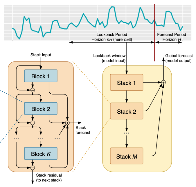
図01
まず時系列データがあり、これがフィルタリングされ、1からMまでの複数のスタックに処理されます。
各スタックは1からKまでの異なるブロックで構成されており、各ブロックからモデルは予測値または残差を出力します。その出力は次のスタックに渡されます。
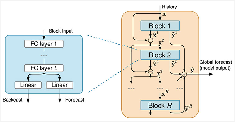
図02
各ブロックは4層の全結合ニューラルネットワークで構成されており、バックキャストまたはフォーキャストを生成します。
モデルへのデータの流れ
01:スタックに
最初に、モデルはルックバック期間と予測期間を設定する必要があります。
ルックバック期間は過去どの範囲を参照して未来を予測するかを示し、予測期間はどのくらい先まで予測するかを示します。
ルックバック期間と予測期間を決定した後、Stack 1にルックバック期間のデータを入力し、初期予測を作成します。たとえば、ルックバック期間が過去数時間のある金融商品の終値であれば、Stack 1はこのデータを使用して次の24時間を予測します。
得られた初期予測とその残差(実際の値 − 予測値)は、次のスタック(Stack 2)に渡され、さらに精緻化されます。
このプロセスは、すべてのスタック(Stack Mまで)で繰り返され、各スタックが前のスタックの予測を改善します。
最終的に、すべてのスタックからの予測を組み合わせてグローバル予測を作成します。たとえば、Stack 1が急上昇を予測し、Stack 2がトレンドを調整し、Stack Mが長期的パターンを修正する場合、グローバル予測はこれらすべての洞察を統合して最も正確な予測を提供します。
スタックは異なる分析層と考えることができます。Stack 1は短期的パターン(例:時間単位の終値の変動)を捉え、Stack 2は長期的パターン(例:日次終値のトレンド)に集中します。
それぞれのスタックは入力データを処理し、全体の予測に独自の貢献をします。
02:入力ブロック内部
Block 1はスタック入力を受け取ります。入力は元のルックバックデータであったり、前のスタックからの残差であったりします。そして、この入力を使用してフォーキャストとバックキャストを生成します。例えば、ブロックが過去24時間の電力使用量を入力として受け取った場合、次の24時間の予測と入力データを近似するバックキャストを生成します。
バックキャストは、予測が全体の予測にどのように貢献するかをモデルが理解するのを助けます。
各スタックは複数のブロックで構成されており、Block 1がスタック入力を処理してフォーキャストとバックキャストを生成した後、次のブロックは前のブロックの残差と元のスタック入力の両方を受け取ります。これにより、現在のブロックは前のブロックよりも正確に予測をおこない、元データを考慮して全体の精度を向上させます。
スタック内の各ブロックでおこなわれるこの反復的な精緻化により、予測はブロックを通じて徐々に正確になります。スタック内のすべてのブロックがデータを処理した後、最後のブロック(Block K)の残差が次のスタックに渡されます。
03:ブロックを解剖する
各ブロック内では、入力データが4層の全結合ネットワークを通して処理されます。このネットワークはブロック入力を変換し、バックキャストとフォーキャストを生成するための特徴量を抽出します。
ブロック内の全結合層はデータ変換と特徴量抽出を担当しており、データが全結合層を通過した後、出力は2つに分かれます(図2)。 1つはバックキャスト用、もう1つは予測用です。
バックキャスト出力は入力データを近似することを目的とし、次のブロックに渡す残差を改善します。一方、フォーキャスト出力は予測期間の予測値を提供します。
PythonでN-BEATSモデルを構築する
まず、記事末の添付表にあるrequirements.txtに記載されているモジュールをすべてインストールします。
pip install -r requirements.txt
次にtest.ipynb内で、必要なモジュールをインポートします。
import MetaTrader5 as mt5
import numpy as np
import matplotlib.pyplot as plt
import pandas as pd
import seaborn as sns
import warnings

sns.set_style("darkgrid")
warnings.filterwarnings("ignore")
続いてMetaTrader 5を初期化します。
if not mt5.initialize():
    print("Metratrader5 initialization failed, Error code =", mt5.last_error())
    mt5.shutdown()
NASDAQ(NAS100)銘柄の日次データから1000本のバーを取得します。
rates = mt5.copy_rates_from_pos("NAS100", mt5.TIMEFRAME_D1, 1, 1000)
rates_df = pd.DataFrame(rates)
このモデルは、従来の機械学習技術でよく使われる多変量手法を応用しているにもかかわらず、N-BEATSはARIMAやVARのような従来の時系列モデルに類似した単変量アプローチを採用しています。
以下のように単変量データを構築します。
univariate_df = rates_df[["time", "close"]].copy()
univariate_df["ds"] = pd.to_datetime(univariate_df["time"], unit="s") # convert the time column to datetime
univariate_df["y"] = univariate_df["close"] # closing prices
univariate_df["unique_id"] = "NAS100" # add a unique_id column | very important for univariate models

# Final dataframe
univariate_df = univariate_df[["unique_id", "ds", "y"]].copy()

univariate_df
以下が出力です。
| unique_id | ds | y | |
|---|---|---|---|
| 0 | NAS100 | 2021-08-30 | 9.655648 |
| 1 | NAS100 | 2021-08-31 | 9.654988 |
| 2 | NAS100 | 2021-09-01 | 9.655763 |
| 3 | NAS100 | 2021-09-02 | 9.654981 |
| 4 | NAS100 | 2021-09-03 | 9.658335 |
| ... | ... | ... | ... |
| 995 | NAS100 | 2025-07-07 | 10.028180 |
| 996 | NAS100 | 2025-07-08 | 10.031142 |
| 997 | NAS100 | 2025-07-09 | 10.037376 |
| 998 | NAS100 | 2025-07-10 | 10.036098 |
| 999 | NAS100 | 2025-07-11 | 10.033283 |
univariate_df["unique_id"] = "NAS100" # add a unique_id column | very important for univariate models
N-BEATSモデルを含むneuralforecastモジュールは、単変量予測とパネル(マルチシリーズ)予測の両方に対応できるよう設計されています。unique_idは各行がどの時系列に属するかをモデルに伝えます。この特徴は特に次の場合に重要です。
- 複数の資産や銘柄(例:AAPL、TSLA、MSFT、EURUSD)を同時に予測する場合
- 複数の時系列に対して単一モデルをバッチ学習させたい場合
単一の時系列であっても、内部のグループ化やインデックス処理のため、この変数は必須です。
モデルの学習は数行のコードで実行できます。
from neuralforecast import NeuralForecast
from neuralforecast.models import NBEATS # Neural Basis Expansion Analysis for Time Series

# Define model and horizon
horizon = 30  # forecast 30 days into the future

model = NeuralForecast(
    models=[NBEATS(h=horizon, # predictive horizon of the model
                   input_size=90, # considered autorregresive inputs (lags), y=[1,2,3,4] input_size=2 -> lags=[1,2].
                   max_steps=100, # maximum number of training steps (epochs)
                   scaler_type='robust', # scaler type for the time series data
                   )],
    freq='D' # frequency of the time series data
)

# Fit the model
model.fit(df=univariate_df)
以下が出力です。
Seed set to 1
GPU available: False, used: False
TPU available: False, using: 0 TPU cores
HPU available: False, using: 0 HPUs

  | Name         | Type          | Params | Mode
-------------------------------------------------------
0 | loss         | MAE           | 0      | train
1 | padder_train | ConstantPad1d | 0      | train
2 | scaler       | TemporalNorm  | 0      | train
3 | blocks       | ModuleList    | 2.6 M  | train
-------------------------------------------------------
2.6 M     Trainable params
7.3 K     Non-trainable params
2.6 M     Total params
10.541    Total estimated model params size (MB)
31        Modules in train mode
0         Modules in eval mode

Epoch 99: 100%
 1/1 [00:01<00:00,  0.88it/s, v_num=32, train_loss_step=0.259, train_loss_epoch=0.259]
`Trainer.fit` stopped: `max_steps=100` reached.
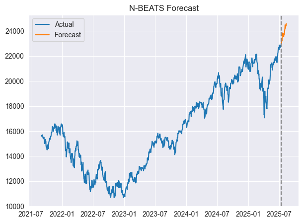
予測値と実際の値を同じ軸上で可視化することも可能です。
forecast = model.predict() # predict future values based on the fitted model

# Merge forecast with original data
plot_df = pd.merge(univariate_df, forecast, on='ds', how='outer')

plt.figure(figsize=(7,5))
plt.plot(plot_df['ds'], plot_df['y'], label='Actual')
plt.plot(plot_df['ds'], plot_df['NBEATS'], label='Forecast')
plt.axvline(plot_df['ds'].max() - pd.Timedelta(days=horizon), color='gray', linestyle='--')
plt.legend()
plt.title('N-BEATS Forecast')
plt.show()
以下が出力です。
マージされたデータフレームの外観は以下の通りです。
| unique_id_x | ds | y | unique_id_y | NBEATS | |
|---|---|---|---|---|---|
| 0 | NAS100 | 2021-08-31 | 15599.4 | NaN | NaN |
| 1 | NAS100 | 2021-09-01 | 15611.5 | NaN | NaN |
| 2 | NAS100 | 2021-09-02 | 15599.3 | NaN | NaN |
| 3 | NAS100 | 2021-09-03 | 15651.7 | NaN | NaN |
| 4 | NAS100 | 2021-09-06 | 15700.4 | NaN | NaN |
| ... | ... | ... | ... | ... | ... |
| 1025 | NaN | 2025-08-09 | NaN | NAS100 | 24235.187500 |
| 1026 | NaN | 2025-08-10 | NaN | NAS100 | 24466.316406 |
| 1027 | NaN | 2025-08-11 | NaN | NAS100 | 24454.646484 |
| 1028 | NaN | 2025-08-12 | NaN | NAS100 | 24405.820312 |
| 1029 | NaN | 2025-08-13 | NaN | NAS100 | 24571.919922 |
これでモデルは30日先までの予測を完了しました。
評価のため、通常の機械学習モデルと同様に、あるデータセットで学習し、別のデータセットでテストすることも可能です。
N-BEATSモデルによるアウトオブサンプル予測
まず、データを学習用とテスト用のデータフレームに分割します。
split_date = '2024-01-01'  # the split date for training and testing

train_df = univariate_df[univariate_df['ds'] < split_date]
test_df = univariate_df[univariate_df['ds'] >= split_date]
次に、学習データでモデルを学習させます。
model = NeuralForecast(
    models=[NBEATS(h=horizon, # predictive horizon of the model
                   input_size=90, # considered autorregresive inputs (lags), y=[1,2,3,4] input_size=2 -> lags=[1,2].
                   max_steps=100, # maximum number of training steps (epochs)
                   scaler_type='robust', # scaler type for the time series data
                   )],
    freq='D' # frequency of the time series data
)

# Fit the model
model.fit(df=train_df)
predict関数は予測期間に応じて次のN日間を予測するため、アウトオブサンプルの評価をおこなうには、予測結果のデータフレームと実際のデータフレームをマージする必要があります。
test_forecast = model.predict() # predict future 30 days based on the training data

df_test = pd.merge(test_df, test_forecast, on=['ds', 'unique_id'], how='outer') # merge the test data with the forecast
df_test.dropna(inplace=True) # drop rows with NaN values

df_test
以下が出力です。
| unique_id | ds | y | NBEATS | |
|---|---|---|---|---|
| 3 | NAS100 | 2024-01-02 | 16554.3 | 16569.835938 |
| 4 | NAS100 | 2024-01-03 | 16368.1 | 16596.839844 |
| 5 | NAS100 | 2024-01-04 | 16287.2 | 16603.513672 |
| 6 | NAS100 | 2024-01-05 | 16307.1 | 16729.607422 |
| 9 | NAS100 | 2024-01-08 | 16631.0 | 16854.746094 |
| 10 | NAS100 | 2024-01-09 | 16672.4 | 16918.466797 |
| 11 | NAS100 | 2024-01-10 | 16804.7 | 16958.833984 |
| 12 | NAS100 | 2024-01-11 | 16814.3 | 17130.972656 |
| 13 | NAS100 | 2024-01-12 | 16808.8 | 17055.396484 |
| 16 | NAS100 | 2024-01-15 | 16828.7 | 17272.376953 |
| 17 | NAS100 | 2024-01-16 | 16841.9 | 17227.498047 |
| 18 | NAS100 | 2024-01-17 | 16727.7 | 17408.158203 |
| 19 | NAS100 | 2024-01-18 | 16987.0 | 17499.619141 |
| 20 | NAS100 | 2024-01-19 | 17336.7 | 17318.767578 |
| 23 | NAS100 | 2024-01-22 | 17329.3 | 17399.562500 |
| 24 | NAS100 | 2024-01-23 | 17426.1 | 17289.140625 |
| 25 | NAS100 | 2024-01-24 | 17503.1 | 17236.478516 |
| 26 | NAS100 | 2024-01-25 | 17469.4 | 17188.691406 |
| 27 | NAS100 | 2024-01-26 | 17390.1 | 17315.134766 |
次に、この結果を評価します。
from sklearn.metrics import mean_absolute_percentage_error, r2_score

mape = mean_absolute_percentage_error(df_test['y'], df_test['NBEATS'])
r2_score_ = r2_score(df_test['y'], df_test['NBEATS'])

print(f"mean_absolute_percentage_error (MAPE): {mape} \n R2 Score: {r2_score_}")
以下が出力です。
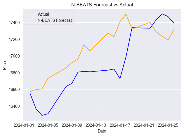
mean_absolute_percentage_error (MAPE): 0.015779373328172166
R2 Score: 0.35350182943487285
MAPE(平均絶対誤差率)の指標によると、モデルの予測は割合として非常に正確です。一方、R²スコアの値が0.35であることは、目的変数の変動のうち35%しか説明できていないことを意味します。
以下は、実際の値と予測値を同じ軸上にプロットした例です。
他の時系列予測モデルと同様に、N-BEATSも新しい連続データが追加されるたびに更新することで、精度を維持できます。前の例では、日次データに基づき30日先の予測でモデルを評価しましたが、この方法では間の多くの日次情報を取りこぼしてしまいます。
正しい方法は、新しいデータが追加されたらすぐにモデルを更新することです。
N-BEATSモデルは、再学習せずに新しいデータでモデルを更新する簡単な方法を提供しており、これにより大幅な時間を節約できます。
以下を実行します。
NBEATS.predict(df=new_dataframe) すると、モデルは、学習済みの重みを新しいデータに適用し、推論をおこないます。これにより、新しいデータフレームから得られた最新情報を取り込み、モデルが最新データに対応できる状態になります。
マルチシリーズ予測
前述のN-BEATSのコアゴールでも説明した通り、 このモデルはマルチシリーズ予測に対応できるよう設計されています。
この能力は非常に優れており、ある時系列で学習したパターンを活用して、他の時系列の予測精度も向上させることができます。
この能力を活用する方法は以下の通りです。
まず、MetaTrader 5から各銘柄のデータを収集します。
rates_nq = mt5.copy_rates_from_pos("NAS100", mt5.TIMEFRAME_D1, 1, 1000)
rates_df_nq = pd.DataFrame(rates_nq)

rates_snp = mt5.copy_rates_from_pos("US500", mt5.TIMEFRAME_D1, 1, 1000)
rates_df_snp = pd.DataFrame(rates_snp)
次に、それぞれの単変量データフレームを準備します。
# NAS100
rates_df_nq["ds"] = pd.to_datetime(rates_df_nq["time"], unit="s")
rates_df_nq["y"] = rates_df_nq["close"]
rates_df_nq["unique_id"] = "NAS100"
df_nq = rates_df_nq[["unique_id", "ds", "y"]]

# US500
rates_df_snp["ds"] = pd.to_datetime(rates_df_snp["time"], unit="s")
rates_df_snp["y"] = rates_df_snp["close"]
rates_df_snp["unique_id"] = "US500"
df_snp = rates_df_snp[["unique_id", "ds", "y"]]
両方のデータフレームを結合し、unique_idと日付順にソートします。
multivariate_df = pd.concat([df_nq, df_snp], ignore_index=True) # combine both dataframes
multivariate_df = multivariate_df.sort_values(['unique_id', 'ds']).reset_index(drop=True) # sort by unique_id and date

multivariate_df
以下が出力です。
| unique_id | ds | y | |
|---|---|---|---|
| 0 | NAS100 | 2021-08-31 | 15599.4 |
| 1 | NAS100 | 2021-09-01 | 15611.5 |
| 2 | NAS100 | 2021-09-02 | 15599.3 |
| 3 | NAS100 | 2021-09-03 | 15651.7 |
| 4 | NAS100 | 2021-09-06 | 15700.4 |
| ... | ... | ... | ... |
| 1995 | US500 | 2025-07-08 | 6229.9 |
| 1996 | US500 | 2025-07-09 | 6264.9 |
| 1997 | US500 | 2025-07-10 | 6280.3 |
| 1998 | US500 | 2025-07-11 | 6255.8 |
| 1999 | US500 | 2025-07-14 | 6271.9 |
前回と同様に、データを学習用とテスト用のデータフレームに分割します。
split_date = '2024-01-01'  # the split date for training and testing

train_df = multivariate_df[multivariate_df['ds'] < split_date]
test_df = multivariate_df[multivariate_df['ds'] >= split_date]
その後、以前と同じ方法でモデルを学習させます。
from neuralforecast import NeuralForecast
from neuralforecast.models import NBEATS # Neural Basis Expansion Analysis for Time Series

# Define model and horizon
horizon = 30  # forecast 30 days into the future

model = NeuralForecast(
    models=[NBEATS(h=horizon, # predictive horizon of the model
                   input_size=90, # considered autorregresive inputs (lags), y=[1,2,3,4] input_size=2 -> lags=[1,2].
                   max_steps=100, # maximum number of training steps (epochs)
                   scaler_type='robust', # scaler type for the time series data
                   )],
    freq='D' # frequency of the time series data
)

# Fit the model
model.fit(df=train_df)
アウトオブサンプルデータに対して予測をおこないます。
test_forecast = model.predict() # predict future 30 days based on the training data

df_test = pd.merge(test_df, test_forecast, on=['ds', 'unique_id'], how='outer') # merge the test data with the forecast
df_test.dropna(inplace=True) # drop rows with NaN values

df_test
以下が出力です。
| unique_id | ds | y | NBEATS | |
|---|---|---|---|---|
| 6 | NAS100 | 2024-01-02 | 16554.3 | 16267.765625 |
| 7 | US500 | 2024-01-02 | 4747.4 | 4706.230957 |
| 8 | NAS100 | 2024-01-03 | 16368.1 | 16230.808594 |
| 9 | US500 | 2024-01-03 | 4707.3 | 4706.517090 |
| 10 | NAS100 | 2024-01-04 | 16287.2 | 16136.568359 |
| 11 | US500 | 2024-01-04 | 4690.9 | 4686.380859 |
| 12 | NAS100 | 2024-01-05 | 16307.1 | 16218.930664 |
| 13 | US500 | 2024-01-05 | 4695.8 | 4704.896484 |
最後に、両方の銘柄でモデルを評価し、実際の値と予測値を同じ軸上で可視化します。
from sklearn.metrics import mean_absolute_percentage_error, r2_score

unique_ids = df_test['unique_id'].unique()

for unique_id in unique_ids:

    df_unique = df_test[df_test['unique_id'] == unique_id].copy()

    mape = mean_absolute_percentage_error(df_unique['y'], df_unique['NBEATS'])
    r2_score_ = r2_score(df_unique['y'], df_unique['NBEATS'])


    print(f"Unique ID: {unique_id} - MAPE: {mape}, R2 Score: {r2_score_}")


    plt.figure(figsize=(7, 4))
    plt.plot(df_unique['ds'], df_unique['y'], label='Actual', color='blue')
    plt.plot(df_unique['ds'], df_unique['NBEATS'], label='Forecast', color='orange')
    plt.title(f'Actual vs Forecast for {unique_id}')
    plt.xlabel('Date')
    plt.ylabel('Value')
    plt.legend()
    plt.show()
以下が出力です。
Unique ID: NAS100 - MAPE: 0.0221775184381915, R2 Score: -0.16976266747298419

Unique ID: US500 - MAPE: 0.007412931117247571, R2 Score: 0.3782229067061038

N-BEATSを使ったMetaTrader 5での取引意思決定
モデルから予測値を取得できるようになったので、Pythonベースの取引ロボットに統合できます。
まず、NBEATS-tradingbot.py内で、モデル全体を最初に学習させる関数を実装します。
def train_nbeats_model(forecast_horizon: int=30,
                       start_bar: int=1,
                       number_of_bars: int=1000,
                       input_size: int=90,
                       max_steps: int=100,
                       mt5_timeframe: int=mt5.TIMEFRAME_D1,
                       symbol_01: str="NAS100",
                       symbol_02: str="US500",
                       test_size_percentage: float=0.2,
                       scaler_type: str='robust'):

    """
        Train NBEATS model on NAS100 and US500 data from MetaTrader 5.

        Args:
            start_bar: starting bar to be used to in CopyRates from MT5
            number_of_bars: The number of bars to extract from MT5 for training the model
            forecast_horizon: the number of days to predict in the future
            input_size: number of previous days to consider for prediction
            max_steps: maximum number of training steps (epochs)
            mt5_timeframe: timeframe to be used for the data extraction from MT5
            symbol_01: unique identifier for the first symbol (default is NAS100)
            symbol_02: unique identifier for the second symbol (default is US500)
            test_size_percentage: percentage of the data to be used for testing (default is 0.2)
            scaler_type: type of scaler to be used for the time series data (default is 'robust')

        Returns:
            NBEATS: the n-beats model object
    """

    # Getting data from MetaTrader 5

    rates_nq = mt5.copy_rates_from_pos(symbol_01, mt5_timeframe, start_bar, number_of_bars)
    rates_df_nq = pd.DataFrame(rates_nq)

    rates_snp = mt5.copy_rates_from_pos(symbol_02, mt5_timeframe, start_bar, number_of_bars)
    rates_df_snp = pd.DataFrame(rates_snp)

    if rates_df_nq.empty or rates_df_snp.empty:
        print(f"Failed to retrieve data for {symbol_01} or {symbol_02}.")
        return None

    # Getting NAS100 data
    rates_df_nq["ds"] = pd.to_datetime(rates_df_nq["time"], unit="s")
    rates_df_nq["y"] = rates_df_nq["close"]
    rates_df_nq["unique_id"] = symbol_01
    df_nq = rates_df_nq[["unique_id", "ds", "y"]]

    # Getting US500 data
    rates_df_snp["ds"] = pd.to_datetime(rates_df_snp["time"], unit="s")
    rates_df_snp["y"] = rates_df_snp["close"]
    rates_df_snp["unique_id"] = symbol_02
    df_snp = rates_df_snp[["unique_id", "ds", "y"]]

    multivariate_df = pd.concat([df_nq, df_snp], ignore_index=True) # combine both dataframes
    multivariate_df = multivariate_df.sort_values(['unique_id', 'ds']).reset_index(drop=True) # sort by unique_id and date

    # Group by unique_id and split per group
    train_df_list = []
    test_df_list = []

    for _, group in multivariate_df.groupby('unique_id'):
        group = group.sort_values('ds')
        split_idx = int(len(group) * (1 - test_size_percentage))

        train_df_list.append(group.iloc[:split_idx])
        test_df_list.append(group.iloc[split_idx:])

    # Concatenate all series
    train_df = pd.concat(train_df_list).reset_index(drop=True)
    test_df = pd.concat(test_df_list).reset_index(drop=True)

    # Define model and horizon

    model = NeuralForecast(
        models=[NBEATS(h=forecast_horizon, # predictive horizon of the model
                    input_size=input_size, # considered autorregresive inputs (lags), y=[1,2,3,4] input_size=2 -> lags=[1,2].
                    max_steps=max_steps, # maximum number of training steps (epochs)
                    scaler_type=scaler_type, # scaler type for the time series data
                    )],
        freq='D' # frequency of the time series data
    )

    # fit the model on the training data

    model.fit(df=train_df)

    test_forecast = model.predict() # predict future 30 days based on the training data

    df_test = pd.merge(test_df, test_forecast, on=['ds', 'unique_id'], how='outer') # merge the test data with the forecast
    df_test.dropna(inplace=True) # drop rows with NaN values


    unique_ids = df_test['unique_id'].unique()
    for unique_id in unique_ids:

        df_unique = df_test[df_test['unique_id'] == unique_id].copy()

        mape = mean_absolute_percentage_error(df_unique['y'], df_unique['NBEATS'])
        print(f"Unique ID: {unique_id} - MAPE: {mape:.2f}")

    return model
この関数は、これまで説明したすべての学習手順を統合しており、直接予測に使えるN-BEATSモデルオブジェクトを返します。
次に、次の値を予測する関数は、学習関数と同様のアプローチで実装されます。
def predict_next(model,
                  symbol_unique_id: str,
                  input_size: int=90):

    """
        Predict the next values for a given unique_id using the trained model.

        Args:
            model (NBEATS): the trained NBEATS model
            symbol_unique_id (str): unique identifier for the symbol to predict
            input_size (int): number of previous days to consider for prediction

        Returns:
            DataFrame: containing the predicted values for the next days
    """

    # Getting data from MetaTrader 5

    rates = mt5.copy_rates_from_pos(symbol_unique_id, mt5.TIMEFRAME_D1, 1, input_size * 2)  # Get enough data for prediction
    if rates is None or len(rates) == 0:
        print(f"Failed to retrieve data for {symbol_unique_id}.")
        return pd.DataFrame()

    rates_df = pd.DataFrame(rates)

    rates_df["ds"] = pd.to_datetime(rates_df["time"], unit="s")
    rates_df = rates_df[["ds", "close"]].rename(columns={"close": "y"})
    rates_df["unique_id"] = symbol_unique_id
    rates_df = rates_df.sort_values(by="ds").reset_index(drop=True)

    # Prepare the dataframe for reference & prediction
    univariate_df = rates_df[["unique_id", "ds", "y"]]
    forecast = model.predict(df=univariate_df)

    return forecast
入力サイズの2倍のデータを渡すのは、学習時に使用したinput_sizeに基づき、十分なデータをモデルに与えるためです。
銘柄ごとにpredict_next関数を呼び出し、結果のデータフレームを確認します。
trained_model = train_nbeats_model(max_steps=10)

print(predict_next(trained_model, "NAS100").head())
print(predict_next(trained_model, "US500").head())
以下が出力です。
Predicting DataLoader 0: 100%|████████████████████████████████████████████████████████████████████████████████████████████████| 1/1 [00:00<00:00, 45.64it/s]
  unique_id         ds        NBEATS
0    NAS100 2025-07-16  22836.160156
1    NAS100 2025-07-17  22931.242188
2    NAS100 2025-07-18  22984.792969
3    NAS100 2025-07-19  23037.224609
4    NAS100 2025-07-20  23119.804688
GPU available: False, used: False
TPU available: False, using: 0 TPU cores
HPU available: False, using: 0 HPUs
Predicting DataLoader 0: 100%|████████████████████████████████████████████████████████████████████████████████████████████████| 1/1 [00:00<00:00, 71.43it/s]
  unique_id         ds       NBEATS
0     US500 2025-07-16  6234.584961
1     US500 2025-07-17  6254.846680
2     US500 2025-07-18  6261.153320
3     US500 2025-07-19  6282.960449
4     US500 2025-07-20  6307.293945
GPU available: False, used: False
TPU available: False, using: 0 TPU cores
HPU available: False, using: 0 HPUs
両銘柄のデータフレームには、30日先までの複数の日次終値予測が含まれているため、今日の日付に対応する値を選択する必要があります(本日の日付は2025年7月16日と仮定)。
today = dt.datetime.now().date() # today's date

forecast_df = predict_next(trained_model, "NAS100") # Get the predicted values for NAS100, 30 days into the future
today_pred_close_nq = forecast_df[forecast_df['ds'].dt.date == today]['NBEATS'].values # extract today's predicted close value for NAS100

forecast_df = predict_next(trained_model, "US500") # Get the predicted values for US500, 30 days into the future
today_pred_close_snp = forecast_df[forecast_df['ds'].dt.date == today]['NBEATS'].values # extract today's predicted close value for US500

print(f"Today's predicted NAS100 values:", today_pred_close_nq)
print(f"Today's predicted US500 values:", today_pred_close_snp)
以下が出力です。
Today's predicted NAS100 values: [22836.16]
Today's predicted US500 values: [6234.585]
最後に、これらの予測値を単純な取引戦略で使用できます。
# Trading modules

from Trade.Trade import CTrade
from Trade.PositionInfo import CPositionInfo
from Trade.SymbolInfo import CSymbolInfo

SLIPPAGE = 100 # points
MAGIC_NUMBER = 15072025 # unique identifier for the trades
TIMEFRAME = mt5.TIMEFRAME_D1 # timeframe for the trades

# Create trade objects for NAS100 and US500
m_trade_nq = CTrade(magic_number=MAGIC_NUMBER,
                 filling_type_symbol = "NAS100",
                 deviation_points=SLIPPAGE)

m_trade_snp = CTrade(magic_number=MAGIC_NUMBER,
                 filling_type_symbol = "US500",
                 deviation_points=SLIPPAGE)

# Training the NBEATS model INITIALLY
trained_model = train_nbeats_model(max_steps=10,
                                    input_size=90,
                                    forecast_horizon=30,
                                    start_bar=1,
                                    number_of_bars=1000,
                                    mt5_timeframe=TIMEFRAME,
                                    symbol_01="NAS100",
                                    symbol_02="US500"
                                   )

m_symbol_nq = CSymbolInfo("NAS100") # Create symbol info object for NAS100
m_symbol_snp = CSymbolInfo("US500") # Create symbol info object for US500

m_position = CPositionInfo() # Create position info object


def pos_exists(pos_type: int, magic: int, symbol: str) -> bool:

    """ Checks whether a position exists given a magic number, symbol, and the position type

    Returns:
        bool: True if a position is found otherwise False
    """

    if mt5.positions_total() < 1: # no positions whatsoever
        return False

    positions = mt5.positions_get()

    for position in positions:
        if m_position.select_position(position):
            if m_position.magic() == magic and m_position.symbol() == symbol and m_position.position_type()==pos_type:
                return True

    return False


def RunStrategyandML(trained_model: NBEATS):

    today = dt.datetime.now().date() # today's date

    forecast_df = predict_next(trained_model, "NAS100") # Get the predicted values for NAS100, 30 days into the future
    today_pred_close_nq = forecast_df[forecast_df['ds'].dt.date == today]['NBEATS'].values # extract today's predicted close value for NAS100

    forecast_df = predict_next(trained_model, "US500") # Get the predicted values for US500, 30 days into the future
    today_pred_close_snp = forecast_df[forecast_df['ds'].dt.date == today]['NBEATS'].values # extract today's predicted close value for US500

    # convert numpy arrays to float values

    today_pred_close_nq = float(today_pred_close_nq[0]) if len(today_pred_close_nq) > 0 else None
    today_pred_close_snp = float(today_pred_close_snp[0]) if len(today_pred_close_snp) > 0 else None

    print(f"Today's predicted NAS100 values:", today_pred_close_nq)
    print(f"Today's predicted US500 values:", today_pred_close_snp)

    # Refreshing the rates for NAS100 and US500 symbols

    m_symbol_nq.refresh_rates()
    m_symbol_snp.refresh_rates()

    ask_price_nq = m_symbol_nq.ask() # get today's close price for NAS100
    ask_price_snp = m_symbol_snp.ask() # get today's close price for US500

    # Trading operations for the NAS100 symol

    if not pos_exists(pos_type=mt5.ORDER_TYPE_BUY, magic=MAGIC_NUMBER, symbol="NAS100"):
        if today_pred_close_nq > ask_price_nq: # if predicted close price for NAS100 is greater than the current ask price
            # Open a buy trade
            m_trade_nq.buy(volume=m_symbol_nq.lots_min(),
                            symbol="NAS100",
                            price=m_symbol_nq.ask(),
                            sl=0.0,
                            tp=today_pred_close_nq) # set take profit to the predicted close price

    print("ask: ", m_symbol_nq.ask(), "bid: ", m_symbol_nq.bid(), "last: ", ask_price_nq)
    print("tp: ", today_pred_close_nq, "lots: ", m_symbol_nq.lots_min())
    print("istp within range: ", (m_symbol_nq.ask() - today_pred_close_nq) > m_symbol_nq.stops_level())

    if not pos_exists(pos_type=mt5.ORDER_TYPE_SELL, magic=MAGIC_NUMBER, symbol="NAS100"):
        if today_pred_close_nq < ask_price_nq: # if predicted close price for NAS100 is less than the current bid price
            m_trade_nq.sell(volume=m_symbol_nq.lots_min(),
                             symbol="NAS100",
                             price=m_symbol_nq.bid(),
                             sl=0.0,
                             tp=today_pred_close_nq) # set take profit to the predicted close price


    # Buy and sell operations for the US500 symbol


    if not pos_exists(pos_type=mt5.ORDER_TYPE_BUY, magic=MAGIC_NUMBER, symbol="US500"):
        if today_pred_close_snp > ask_price_snp: # if the predicted price for US500 is greater than the current ask price
            m_trade_snp.buy(volume=m_symbol_snp.lots_min(),
                            symbol="US500",
                            price=m_symbol_snp.ask(),
                            sl=0.0,
                            tp=today_pred_close_snp)

    if not pos_exists(pos_type=mt5.ORDER_TYPE_SELL, magic=MAGIC_NUMBER, symbol="US500"):
        if today_pred_close_snp < ask_price_snp: # if the predicted price for US500 is less than the current bid price
            m_trade_snp.sell(volume=m_symbol_snp.lots_min(),
                             symbol="US500",
                             price=m_symbol_snp.bid(),
                             sl=0.0,
                             tp=today_pred_close_snp)


RunStrategyandML(trained_model=trained_model) # Run the strategy and ML model once to initialize
以下が出力です。
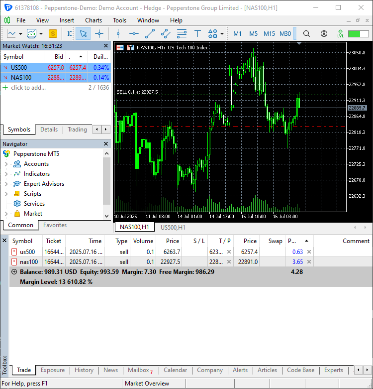
2つの新しい取引が開始されました。
最後に、学習の進行をスケジュール化し、モデルが毎日の開始時に自動で予測をおこない、エントリーできるように自動化します。
# Schedule the strategy to run every day at 00:00
schedule.every().day.at("00:00").do(RunStrategyandML, trained_model=trained_model)

while True:

    schedule.run_pending()
    time.sleep(10)
結論
N-BEATSは、時系列分析と予測のための強力なモデルです。ARIMA、VAR、PROPHETなどの従来モデルを同じタスクで上回ることができる理由は、複雑なパターンを捉えることに優れたニューラルネットワークを核として活用している点にあります。
N-BEATSは、従来型の時系列予測モデルに頼らず、非伝統的なモデルで時系列予測をおこないたい人にとって、非常に適した代替手段です。
特に、正規化手法や評価ツールがツールボックスに含まれているため、使いやすさも魅力です。
しかし、どの機械学習モデルにも言えることですが、N-BEATSにも認識すべき欠点があります。
- 主に単変量予測用に設計されている
前述の通り、学習用データフレームでは主にds(日付)と目的変数yの2つの特徴量だけが必要です。これは、以前に紹介したPROPHETモデルと同様です。
金融データにおいては、この2つの特徴量だけでは市場のダイナミクスを十分に捉えることはできません。 - ノイズの多いデータに過剰適合する可能性がある
他のディープネットワーク同様、N-BEATSもノイズの多いデータで過学習する可能性があります。 - 解釈性が限定的
N-BEATSは解釈性のための基底関数分解を含みますが、あくまでディープニューラルネットワークであるため、ARIMAやPROPHETのような時系列予測モデルと比べると解釈性は低くなります。 - 産業界での採用例が少ない
おそらく、このモデルの名前を聞いたことがない方も多いでしょう。
学術的なベンチマークでは強力ですが、ARIMA、XGBoost、LSTMなどと比べると、機械学習コミュニティでの採用例は少なく、オンラインでもこのモデルに関する情報はあまり多くありません。
ご一読、誠にありがとうございました。
添付ファイルの表
| ファイル名 | 説明と使用法 |
|---|---|
| Trade\PositionInfo.py | MQL5で提供されるものと同様のCPositionInfoクラスを含むファイル。MetaTrader 5で開かれているすべてのポジション情報を提供 |
| Trade\SymbolInfo.py | MQL5で提供されるものと同様のCSymbolInfoクラスを含むファイル。MetaTrader 5で選択された銘柄に関するすべての情報を提供 |
| Trade\Trade.py | MQL5で提供されるものと同様のCTradeクラスを含むファイル。MetaTrader 5での取引のオープンやクローズの関数を提供 |
| error_description.py | MetaTrader 5のエラーコードを人間が読みやすい情報に変換する関数 |
| NBEATS-Tradingbot.py | N-BEATSモデルを用いて取引意思決定をおこなうPythonスクリプトです。 |
| test.ipynb | N-BEATSモデルを試すためのJupyter Notebook |
| requirements.txt | 本プロジェクトで使用されるPython依存関係をすべて記載したファイルです。 |
情報源と参考文献
MetaQuotes Ltdにより英語から翻訳されました。
元の記事: https://www.mql5.com/en/articles/18242
警告: これらの資料についてのすべての権利はMetaQuotes Ltd.が保有しています。これらの資料の全部または一部の複製や再プリントは禁じられています。
この記事はサイトのユーザーによって執筆されたものであり、著者の個人的な見解を反映しています。MetaQuotes Ltdは、提示された情報の正確性や、記載されているソリューション、戦略、または推奨事項の使用によって生じたいかなる結果についても責任を負いません。

- 無料取引アプリ
- 8千を超えるシグナルをコピー
- 金融ニュースで金融マーケットを探索
新しい記事をご覧ください:データサイエンスとML (第46回):PythonでN-BEATSを使った株式市場予測。
著者オメガ・J・ミシグワ