基于时间、价格和成交量创建 3D 柱状图引入波动率测量

引言

这个项目我已经做了六个月了。从那个最初看起来很蠢的想法开始，所以我没有太投入，只是和一些熟悉的交易者讨论过。 

一切都始于一个简单的问题——为什么交易员们总是试图通过二维图表来分析三维市场？价格行为、技术分析、波浪理论——所有这些都是在将市场投影到平面上进行分析。但如果我们尝试看到价格、成交量和时间的真实结构呢？

在我研究算法系统的过程中，我不断发现传统指标忽略了价格和成交量之间的关键关系。

3D 柱状图的想法并不是一下子就出现的。一开始，我尝试对市场深度进行三维可视化实验。然后出现了成交量-价格集群的初步草图。当我加入时间维度并构建出第一个 3D 柱状图时，很明显，这是一种全新的看待市场的方式。

今天我想与大家分享这项工作的成果。我将展示 Python 和 MetaTrader 5 如何让你实时构建成交量柱状图。我将介绍计算背后的数学原理，以及如何在实战交易中使用这些信息。

3D 柱状图有什么不同？

只要我们通过二维图表来观察市场，我们就会错过最重要的一点——市场的真实结构。传统技术分析处理的是价格-时间、成交量-时间的投影，但从未展示这些组件相互作用的完整图景。

3D 分析的根本不同之处在于它让我们能够整体地看待市场。当我们构建一个成交量柱形时，我们实际上是在创建市场状态的“快照”，其中每个维度都承载着关键信息：

• 柱的高度显示价格波动的幅度
• 宽度反映时间尺度
• 深度可视化成交量分布

为什么它很重要？想象一下图表上两个完全相同的价格走势。在二维中它们看起来一模一样。但当我们加入成交量维度后，情况就大不相同了——一个走势可能得到大量成交量的支持，形成一个深厚而稳定的柱，而另一个则可能只是表面上的波动，几乎没有真实交易的支持。

使用 3D 柱状图的综合方法解决了技术分析的一个经典问题——信号滞后。柱的体积结构从第一笔 tick 就开始形成，让我们能够在常规图表上出现之前很久就看到强劲走势的出现。本质上，我们获得了一个预测分析工具，它不是基于历史模式，而是基于当前交易的真实动态。

多元数据分析不仅仅是漂亮的可视化；它是一种理解市场微观结构的全新方式。每一个 3D 柱都包含以下信息：

• 价格区间内的成交量分布
• 头寸积累速度
• 买卖双方的不平衡
• 微观层面的波动性
• 走势的动量

所有这些组件作为一个整体机制运作，让你能够看到价格走势的真实本质。在传统技术分析只看到一根K线或柱状图的地方，3D 分析展示了供需相互作用的复杂结构。

计算主要指标的方程。构建 7D 柱的基本原则。将不同维度组合成单一系统的逻辑

3D 柱的数学模型源于对真实市场微观结构的分析。系统中的每个柱都可以表示为一个三维图形，其中：

class Bar3D:
    def __init__(self):
        self.price_range = None  # Price range
        self.time_period = None  # Time interval
        self.volume_profile = {} # Volume profile by prices
        self.direction = None    # Movement direction
        self.momentum = None     # Impulse
        self.volatility = None   # Volatility
        self.spread = None       # Average spread

关键点在于柱形内部体积分布的计算。与传统柱不同，我们分析的是成交量在价格水平上的分布。

def calculate_volume_profile(self, ticks_data):
    volume_by_price = defaultdict(float)
    
    for tick in ticks_data:
        price_level = round(tick.price, 5)
        volume_by_price[price_level] += tick.volume
        
    # Normalize the profile
    total_volume = sum(volume_by_price.values())
    for price in volume_by_price:
        volume_by_price[price] /= total_volume
        
    return volume_by_price

动量计算为价格变化率和成交量的组合：

def calculate_momentum(self):
    price_velocity = (self.close - self.open) / self.time_period
    volume_intensity = self.total_volume / self.time_period
    self.momentum = price_velocity * volume_intensity * self.direction

特别关注柱内波动率的分析。我们使用一种修正的 ATR 公式，考虑了走势的微观结构：

def calculate_volatility(self, tick_data):
    tick_changes = np.diff([tick.price for tick in tick_data])
    weighted_std = np.std(tick_changes * [tick.volume for tick in tick_data[1:]])
    time_factor = np.sqrt(self.time_period)
    self.volatility = weighted_std * time_factor

与传统柱形的根本区别在于所有指标都是实时计算的，让我们能够看到柱结构的形成：

def update_bar(self, new_tick):
    self.update_price_range(new_tick.price)
    self.update_volume_profile(new_tick)
    self.recalculate_momentum()
    self.update_volatility(new_tick)
    
    # Recalculate the volumetric center of gravity
    self.volume_poc = self.calculate_poc()

所有测量通过一个权重系统组合，权重根据具体品种调整：

def calculate_bar_strength(self):
    return (self.momentum_weight * self.normalized_momentum +
            self.volatility_weight * self.normalized_volatility +
            self.volume_weight * self.normalized_volume_concentration +
            self.spread_weight * self.normalized_spread_factor)

在实际交易中，这个数学模型让我们能够看到市场的以下方面：

• 成交量积累的不平衡
• 价格形成速度的异常
• 盘整与突破区域
• 通过成交量特征判断趋势的真实强度

每一个 3D 柱形不再是图表上的一个点，而是特定时刻市场状态的完整指标。

创建 3D 柱的算法详细分析。使用 MetaTrader 5 的特点。数据处理细节

调试完主算法后，我终于到了最有趣的部分——实时实现多维柱。我承认，一开始这似乎是一项艰巨的任务。MetaTrader 5 对外部脚本不太友好，文档有时也未能提供充分的理解。但让我告诉你我是如何最终克服这些困难的。

我从存储数据的基本结构开始。经过几次迭代，诞生了以下类：

class Bar7D:
    def __init__(self):
        self.time = None
        self.open = None
        self.high = None
        self.low = None
        self.close = None
        self.tick_volume = 0
        self.volume_profile = {}
        self.direction = 0
        self.trend_count = 0
        self.volatility = 0
        self.momentum = 0

最困难的部分是弄清楚如何正确计算块大小。经过大量实验，我确定了以下公式：

def calculate_brick_size(symbol_info, multiplier=45):
    spread = symbol_info.spread
    point = symbol_info.point
    min_price_brick = spread * multiplier * point
    
    # Adaptive adjustment for volatility
    atr = calculate_atr(symbol_info.name)
    if atr > min_price_brick * 2:
        min_price_brick = atr / 2
        
    return min_price_brick

成交量也给我带来了很多麻烦。起初，我想使用固定大小的 volume_brick，但很快意识到这行不通。解决方案来自一个自适应算法：

def adaptive_volume_threshold(tick_volume, history_volumes):
    median_volume = np.median(history_volumes)
    std_volume = np.std(history_volumes)
    
    if tick_volume > median_volume + 2 * std_volume:
        return median_volume + std_volume
    return max(tick_volume, median_volume / 2)

但我想我在统计指标的计算上有点过度了：

def calculate_stats(df):
    df['ma_5'] = df['close'].rolling(5).mean()
    df['ma_20'] = df['close'].rolling(20).mean()
    df['volume_ma_5'] = df['tick_volume'].rolling(5).mean()
    df['price_volatility'] = df['price_change'].rolling(10).std()
    df['volume_volatility'] = df['tick_volume'].rolling(10).std()
    df['trend_strength'] = df['trend_count'] * df['direction']
    
    # This is probably too much
    df['zscore_price'] = stats.zscore(df['close'], nan_policy='omit')
    df['zscore_volume'] = stats.zscore(df['tick_volume'], nan_policy='omit')
    return df

有趣的是，最困难的部分不是写代码，而是在实际条件下调试它。 

这是最终函数的结果，特点是归一化范围在 3-9 之间。为什么是 3-9？江恩和特斯拉都声称这些数字中隐藏着某种魔力。我也亲眼见过一个知名平台上的交易员，他声称基于这些数字创建了一个成功的反转脚本。但我们还是不要深入阴谋论和神秘主义。不如试试这个：

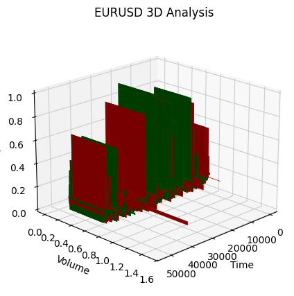
def create_true_3d_renko(symbol, timeframe, min_spread_multiplier=45, volume_brick=500, lookback=20000):
    """
    Creates 3D Renko bars with extended analytics
    """
    rates = mt5.copy_rates_from_pos(symbol, timeframe, 0, lookback)
    if rates is None:
        print(f"Error getting data for {symbol}")
        return None, None
        
    df = pd.DataFrame(rates)
    df['time'] = pd.to_datetime(df['time'], unit='s')
    
    if df.isnull().any().any():
        print("Missing values detected, cleaning...")
        df = df.dropna()
        if len(df) == 0:
            print("No data for analysis after cleaning")
            return None, None
    
    symbol_info = mt5.symbol_info(symbol)
    if symbol_info is None:
        print(f"Failed to get symbol info for {symbol}")
        return None, None
    
    try:
        min_price_brick = symbol_info.spread * min_spread_multiplier * symbol_info.point
        if min_price_brick <= 0:
            print("Invalid block size")
            return None, None
    except AttributeError as e:
        print(f"Error getting symbol parameters: {e}")
        return None, None
    
    # Convert time to numeric and scale everything
    scaler = MinMaxScaler(feature_range=(3, 9))
    
    # Convert datetime to numeric (seconds from start)
    df['time_numeric'] = (df['time'] - df['time'].min()).dt.total_seconds()
    
    # Scale all numeric data together
    columns_to_scale = ['time_numeric', 'open', 'high', 'low', 'close', 'tick_volume']
    df[columns_to_scale] = scaler.fit_transform(df[columns_to_scale])
    
    renko_blocks = []
    current_price = float(df.iloc[0]['close'])
    current_tick_volume = 0
    current_time = df.iloc[0]['time']
    current_time_numeric = float(df.iloc[0]['time_numeric'])
    current_spread = float(symbol_info.spread)
    current_type = 0
    prev_direction = 0
    trend_count = 0
    
    try:
        for idx, row in df.iterrows():
            if pd.isna(row['tick_volume']) or pd.isna(row['close']):
                continue
                
            current_tick_volume += float(row['tick_volume'])
            volume_bricks = int(current_tick_volume / volume_brick)
            
            price_diff = float(row['close']) - current_price
            if pd.isna(price_diff) or pd.isna(min_price_brick):
                continue
                
            price_bricks = int(price_diff / min_price_brick)
            
            if volume_bricks > 0 or abs(price_bricks) > 0:
                direction = np.sign(price_bricks) if price_bricks != 0 else 1
                
                if direction == prev_direction:
                    trend_count += 1
                else:
                    trend_count = 1
                
                renko_block = {
                    'time': current_time,
                    'time_numeric': float(row['time_numeric']),
                    'open': float(row['open']),
                    'close': float(row['close']),
                    'high': float(row['high']),
                    'low': float(row['low']),
                    'tick_volume': float(row['tick_volume']),
                    'direction': float(direction),
                    'spread': float(current_spread),
                    'type': float(current_type),
                    'trend_count': trend_count,
                    'price_change': price_diff,
                    'volume_intensity': float(row['tick_volume']) / volume_brick,
                    'price_velocity': price_diff / (volume_bricks if volume_bricks > 0 else 1)
                }
                
                if volume_bricks > 0:
                    current_tick_volume = current_tick_volume % volume_brick
                if price_bricks != 0:
                    current_price += min_price_brick * price_bricks
                    
                prev_direction = direction
                renko_blocks.append(renko_block)
                
    except Exception as e:
        print(f"Error processing data: {e}")
        if len(renko_blocks) == 0:
            return None, None
    
    if len(renko_blocks) == 0:
        print("Failed to create any blocks")
        return None, None
        
    result_df = pd.DataFrame(renko_blocks)
    
    # Scale derived metrics to same range
    derived_metrics = ['price_change', 'volume_intensity', 'price_velocity', 'spread']
    result_df[derived_metrics] = scaler.fit_transform(result_df[derived_metrics])
    
    # Add analytical metrics using scaled data
    result_df['ma_5'] = result_df['close'].rolling(5).mean()
    result_df['ma_20'] = result_df['close'].rolling(20).mean()
    result_df['volume_ma_5'] = result_df['tick_volume'].rolling(5).mean()
    result_df['price_volatility'] = result_df['price_change'].rolling(10).std()
    result_df['volume_volatility'] = result_df['tick_volume'].rolling(10).std()
    result_df['trend_strength'] = result_df['trend_count'] * result_df['direction']
    
    # Scale moving averages and volatility
    ma_columns = ['ma_5', 'ma_20', 'volume_ma_5', 'price_volatility', 'volume_volatility', 'trend_strength']
    result_df[ma_columns] = scaler.fit_transform(result_df[ma_columns])
    
    # Add statistical metrics and scale them
    result_df['zscore_price'] = stats.zscore(result_df['close'], nan_policy='omit')
    result_df['zscore_volume'] = stats.zscore(result_df['tick_volume'], nan_policy='omit')
    zscore_columns = ['zscore_price', 'zscore_volume']
    result_df[zscore_columns] = scaler.fit_transform(result_df[zscore_columns])
    
    return result_df, min_price_brick

这就是我们在单一尺度上获得的一系列柱状图的样子。看起来不太平稳，对吧？

统计分布：

 

自然，我对这样的序列并不满意，因为我的目标是创建一个或多或少平稳的序列——一个平稳的时间-成交量-价格序列。下面是我接下来所做的：

引入波动率度量 

在实现 create_stationary_4d_features 函数时，我采取了一条根本不同的路径。与原始的 3D 柱状图不同——在原始方法中我们只是将数据缩放到 3-9 的范围——在这里，我专注于创建真正平稳的序列。

该函数的核心思想是通过平稳特征来创建市场的四维表示。不是简单地进行缩放，而是对每个维度进行特殊变换，以实现平稳性：

1. 时间维度：这里我应用了三角变换，将小时数转换为正弦和余弦波。sin(2π * hour/24) 和 cos(2π * hour/24) 这两个公式创建了周期性特征，完全消除了每日季节性问题。
2. 价格测量：不使用绝对价格值，而是使用它们的相对变化。在代码中，这是通过计算典型价格 (high + low + close)/3，然后计算其回报率及其加速度来实现的。这种方法使得序列在任意价格水平下都能保持平稳。
3. 成交量测量：这里有个有趣的点——我们不只是用成交量的变化，而是用它们的相对增量。这很重要，因为成交量通常分布非常不均匀。在代码中，这是通过连续应用 pct_change() 和 diff() 来实现的。
4. 波动率测量：这里我实现了一个两步变换——首先通过回报率的标准差计算滚动波动率，然后取该波动率的相对变化。实际上，我们得到的是“波动率的波动率”。

每个数据块都是在 20 个周期的滑动窗口中形成的。这不是一个随机数字——它是在保留数据局部结构和确保计算统计显著性之间做出的折中选择。

所有计算出的特征最终都会被缩放到 3-9 的范围，但这只是对已经平稳的序列进行的二次变换。这使我们能够在使用根本不同的数据预处理方法的同时，保持与原始 3D 柱状图实现的兼容性。

一个特别重要的点是保留原始函数中的所有关键指标——移动平均线、波动率、z 分数。这使得新的实现可以直接替代原始函数，同时获得更高质量的平稳数据。

最终，我们获得了一组不仅在统计意义上平稳，还保留了市场结构所有重要信息的特征。这种方法使数据更适合应用机器学习和统计分析方法，同时仍保持其与原始交易情境的联系。

这个函数如下： 

def create_true_3d_renko(symbol, timeframe, min_spread_multiplier=45, volume_brick=500, lookback=20000):
    """
    Creates 4D stationary features with same interface as 3D Renko
    """
    rates = mt5.copy_rates_from_pos(symbol, timeframe, 0, lookback)
    if rates is None:
        print(f"Error getting data for {symbol}")
        return None, None
        
    df = pd.DataFrame(rates)
    df['time'] = pd.to_datetime(df['time'], unit='s')
    
    if df.isnull().any().any():
        print("Missing values detected, cleaning...")
        df = df.dropna()
        if len(df) == 0:
            print("No data for analysis after cleaning")
            return None, None
    
    symbol_info = mt5.symbol_info(symbol)
    if symbol_info is None:
        print(f"Failed to get symbol info for {symbol}")
        return None, None
    
    try:
        min_price_brick = symbol_info.spread * min_spread_multiplier * symbol_info.point
        if min_price_brick <= 0:
            print("Invalid block size")
            return None, None
    except AttributeError as e:
        print(f"Error getting symbol parameters: {e}")
        return None, None
    
    scaler = MinMaxScaler(feature_range=(3, 9))
    df_blocks = []
    
    try:
        # Time dimension
        df['time_sin'] = np.sin(2 * np.pi * df['time'].dt.hour / 24)
        df['time_cos'] = np.cos(2 * np.pi * df['time'].dt.hour / 24)
        df['time_numeric'] = (df['time'] - df['time'].min()).dt.total_seconds()
        
        # Price dimension
        df['typical_price'] = (df['high'] + df['low'] + df['close']) / 3
        df['price_return'] = df['typical_price'].pct_change()
        df['price_acceleration'] = df['price_return'].diff()
        
        # Volume dimension
        df['volume_change'] = df['tick_volume'].pct_change()
        df['volume_acceleration'] = df['volume_change'].diff()
        
        # Volatility dimension
        df['volatility'] = df['price_return'].rolling(20).std()
        df['volatility_change'] = df['volatility'].pct_change()
        
        for idx in range(20, len(df)):
            window = df.iloc[idx-20:idx+1]
            
            block = {
                'time': df.iloc[idx]['time'],
                'time_numeric': scaler.fit_transform([[float(df.iloc[idx]['time_numeric'])]]).item(),
                'open': float(window['price_return'].iloc[-1]),
                'high': float(window['price_acceleration'].iloc[-1]),
                'low': float(window['volume_change'].iloc[-1]),
                'close': float(window['volatility_change'].iloc[-1]),
                'tick_volume': float(window['volume_acceleration'].iloc[-1]),
                'direction': np.sign(window['price_return'].iloc[-1]),
                'spread': float(df.iloc[idx]['time_sin']),
                'type': float(df.iloc[idx]['time_cos']),
                'trend_count': len(window),
                'price_change': float(window['price_return'].mean()),
                'volume_intensity': float(window['volume_change'].mean()),
                'price_velocity': float(window['price_acceleration'].mean())
            }
            df_blocks.append(block)
                
    except Exception as e:
        print(f"Error processing data: {e}")
        if len(df_blocks) == 0:
            return None, None
    
    if len(df_blocks) == 0:
        print("Failed to create any blocks")
        return None, None
        
    result_df = pd.DataFrame(df_blocks)
    
    # Scale all features
    features_to_scale = [col for col in result_df.columns if col != 'time' and col != 'direction']
    result_df[features_to_scale] = scaler.fit_transform(result_df[features_to_scale])
    
    # Add same analytical metrics as in original function
    result_df['ma_5'] = result_df['close'].rolling(5).mean()
    result_df['ma_20'] = result_df['close'].rolling(20).mean()
    result_df['volume_ma_5'] = result_df['tick_volume'].rolling(5).mean()
    result_df['price_volatility'] = result_df['price_change'].rolling(10).std()
    result_df['volume_volatility'] = result_df['tick_volume'].rolling(10).std()
    result_df['trend_strength'] = result_df['trend_count'] * result_df['direction']
    
    # Scale moving averages and volatility
    ma_columns = ['ma_5', 'ma_20', 'volume_ma_5', 'price_volatility', 'volume_volatility', 'trend_strength']
    result_df[ma_columns] = scaler.fit_transform(result_df[ma_columns])
    
    # Add statistical metrics and scale them
    result_df['zscore_price'] = stats.zscore(result_df['close'], nan_policy='omit')
    result_df['zscore_volume'] = stats.zscore(result_df['tick_volume'], nan_policy='omit')
    zscore_columns = ['zscore_price', 'zscore_volume']
    result_df[zscore_columns] = scaler.fit_transform(result_df[zscore_columns])
    
    return result_df, min_price_brick

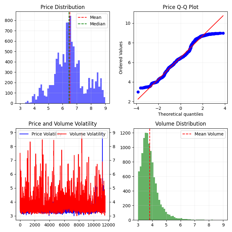
这是T它在2D模式下的样子：

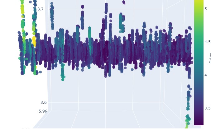
接下来，让我们尝试使用 plotly 为三维价格数据创建一个交互式 3D 模型。附近应该可以看到一个常规的二维图表。代码如下：

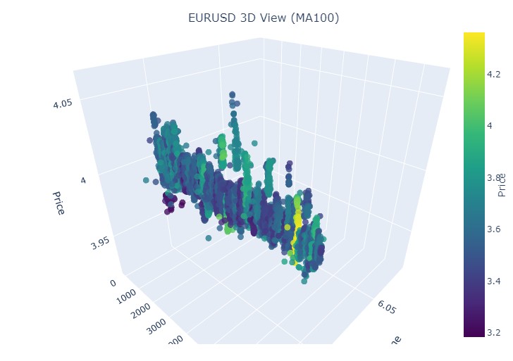
import plotly.graph_objects as go
from plotly.subplots import make_subplots


def create_interactive_3d(df, symbol, save_dir):
    """
    Creates interactive 3D visualization with smoothed data and original price chart
    """
    try:
        save_dir = Path(save_dir)
        
        # Smooth all series with MA(100)
        df_smooth = df.copy()
        smooth_columns = ['close', 'tick_volume', 'price_volatility', 'volume_volatility']
        
        for col in smooth_columns:
            df_smooth[f'{col}_smooth'] = df_smooth[col].rolling(window=100, min_periods=1).mean()
        
        # Create subplots: 3D view and original chart side by side
        fig = make_subplots(
            rows=1, cols=2,
            specs=[[{'type': 'scene'}, {'type': 'xy'}]],
            subplot_titles=(f'{symbol} 3D View (MA100)', f'{symbol} Original Price'),
            horizontal_spacing=0.05
        )
        
        # Add 3D scatter plot
        fig.add_trace(
            go.Scatter3d(
                x=np.arange(len(df_smooth)),
                y=df_smooth['tick_volume_smooth'],
                z=df_smooth['close_smooth'],
                mode='markers',
                marker=dict(
                    size=5,
                    color=df_smooth['price_volatility_smooth'],
                    colorscale='Viridis',
                    opacity=0.8,
                    showscale=True,
                    colorbar=dict(x=0.45)
                ),
                hovertemplate=
                "Time: %{x}<br>" +
                "Volume: %{y:.2f}<br>" +
                "Price: %{z:.5f}<br>" +
                "Volatility: %{marker.color:.5f}",
                name='3D View'
            ),
            row=1, col=1
        )
        
        # Add original price chart
        fig.add_trace(
            go.Candlestick(
                x=np.arange(len(df)),
                open=df['open'],
                high=df['high'],
                low=df['low'],
                close=df['close'],
                name='OHLC'
            ),
            row=1, col=2
        )
        
        # Add smoothed price line
        fig.add_trace(
            go.Scatter(
                x=np.arange(len(df_smooth)),
                y=df_smooth['close_smooth'],
                line=dict(color='blue', width=1),
                name='MA100'
            ),
            row=1, col=2
        )
        
        # Update 3D layout
        fig.update_scenes(
            xaxis_title='Time',
            yaxis_title='Volume',
            zaxis_title='Price',
            camera=dict(
                up=dict(x=0, y=0, z=1),
                center=dict(x=0, y=0, z=0),
                eye=dict(x=1.5, y=1.5, z=1.5)
            )
        )
        
        # Update 2D layout
        fig.update_xaxes(title_text="Time", row=1, col=2)
        fig.update_yaxes(title_text="Price", row=1, col=2)
        
        # Update overall layout
        fig.update_layout(
            width=1500,  # Double width to accommodate both plots
            height=750,
            showlegend=True,
            title_text=f"{symbol} Combined Analysis"
        )
        
        # Save interactive HTML
        fig.write_html(save_dir / f'{symbol}_combined_view.html')
        
        # Create additional plots with smoothed data (unchanged)
        fig2 = make_subplots(rows=2, cols=2, 
                            subplot_titles=('Smoothed Price', 'Smoothed Volume',
                                          'Smoothed Price Volatility', 'Smoothed Volume Volatility'))
        
        fig2.add_trace(
            go.Scatter(x=np.arange(len(df_smooth)), y=df_smooth['close_smooth'],
                      name='Price MA100'),
            row=1, col=1
        )
        
        fig2.add_trace(
            go.Scatter(x=np.arange(len(df_smooth)), y=df_smooth['tick_volume_smooth'],
                      name='Volume MA100'),
            row=1, col=2
        )
        
        fig2.add_trace(
            go.Scatter(x=np.arange(len(df_smooth)), y=df_smooth['price_volatility_smooth'],
                      name='Price Vol MA100'),
            row=2, col=1
        )
        
        fig2.add_trace(
            go.Scatter(x=np.arange(len(df_smooth)), y=df_smooth['volume_volatility_smooth'],
                      name='Volume Vol MA100'),
            row=2, col=2
        )
        
        fig2.update_layout(
            height=750,
            width=750,
            showlegend=True,
            title_text=f"{symbol} Smoothed Data Analysis"
        )
        
        fig2.write_html(save_dir / f'{symbol}_smoothed_analysis.html')
        
        print(f"Interactive visualizations saved in {save_dir}")
        
    except Exception as e:
        print(f"Error creating interactive visualization: {e}")
        raise

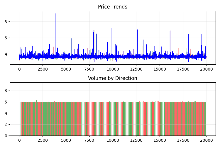
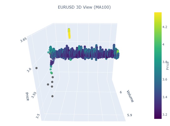
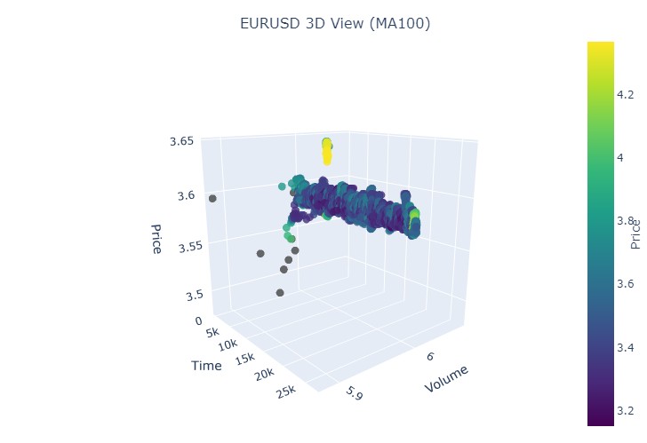
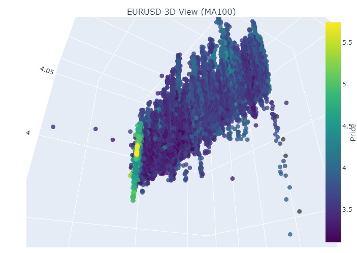
这就是我们新的价格范围的样子：

总体来看，它看起来非常有趣。我们看到了按时间分组的价格序列，以及按成交量分组的价格离群值。因此，产生了一种感觉（并且也直接得到了顶尖交易员的经验证实）：当市场不安定、当大量资金被抛出、当波动性急剧上升时，我们正在面对一种超出统计范围的危险爆发——也就是那臭名昭著的尾部风险。因此，在这里我们可以立即检测到价格在这种坐标上的“异常”偏离。仅凭这一点，我就想感谢多元价格图表这一构想！ 

请注意：

检查“问题对象”（3D 图形）

接下来，我建议进行可视化。但不是在棕榈树下想象我们的美好未来，而是对 3D 价格图表进行可视化。我们将这些情况分为三类：上升趋势、下降趋势、从上升趋势转为下降趋势的反转，以及从下降趋势转为上升趋势的反转。为此，我们需要稍微修改代码：我们不再需要柱状图的索引，我们将加载特定日期的数据。实际上，要做到这一点，我们只需要使用 mt5.copy_rates_range 即可。

def create_true_3d_renko(symbol, timeframe, start_date, end_date, min_spread_multiplier=45, volume_brick=500):
    """
    Creates 4D stationary features with same interface as 3D Renko
    """
    rates = mt5.copy_rates_range(symbol, timeframe, start_date, end_date)
    if rates is None:
        print(f"Error getting data for {symbol}")
        return None, None
        
    df = pd.DataFrame(rates)
    df['time'] = pd.to_datetime(df['time'], unit='s')
    
    if df.isnull().any().any():
        print("Missing values detected, cleaning...")
        df = df.dropna()
        if len(df) == 0:
            print("No data for analysis after cleaning")
            return None, None
    
    symbol_info = mt5.symbol_info(symbol)
    if symbol_info is None:
        print(f"Failed to get symbol info for {symbol}")
        return None, None
    
    try:
        min_price_brick = symbol_info.spread * min_spread_multiplier * symbol_info.point
        if min_price_brick <= 0:
            print("Invalid block size")
            return None, None
    except AttributeError as e:
        print(f"Error getting symbol parameters: {e}")
        return None, None
    
    scaler = MinMaxScaler(feature_range=(3, 9))
    df_blocks = []
    
    try:
        # Time dimension
        df['time_sin'] = np.sin(2 * np.pi * df['time'].dt.hour / 24)
        df['time_cos'] = np.cos(2 * np.pi * df['time'].dt.hour / 24)
        df['time_numeric'] = (df['time'] - df['time'].min()).dt.total_seconds()
        
        # Price dimension
        df['typical_price'] = (df['high'] + df['low'] + df['close']) / 3
        df['price_return'] = df['typical_price'].pct_change()
        df['price_acceleration'] = df['price_return'].diff()
        
        # Volume dimension
        df['volume_change'] = df['tick_volume'].pct_change()
        df['volume_acceleration'] = df['volume_change'].diff()
        
        # Volatility dimension
        df['volatility'] = df['price_return'].rolling(20).std()
        df['volatility_change'] = df['volatility'].pct_change()
        
        for idx in range(20, len(df)):
            window = df.iloc[idx-20:idx+1]
            
            block = {
                'time': df.iloc[idx]['time'],
                'time_numeric': scaler.fit_transform([[float(df.iloc[idx]['time_numeric'])]]).item(),
                'open': float(window['price_return'].iloc[-1]),
                'high': float(window['price_acceleration'].iloc[-1]),
                'low': float(window['volume_change'].iloc[-1]),
                'close': float(window['volatility_change'].iloc[-1]),
                'tick_volume': float(window['volume_acceleration'].iloc[-1]),
                'direction': np.sign(window['price_return'].iloc[-1]),
                'spread': float(df.iloc[idx]['time_sin']),
                'type': float(df.iloc[idx]['time_cos']),
                'trend_count': len(window),
                'price_change': float(window['price_return'].mean()),
                'volume_intensity': float(window['volume_change'].mean()),
                'price_velocity': float(window['price_acceleration'].mean())
            }
            df_blocks.append(block)
                
    except Exception as e:
        print(f"Error processing data: {e}")
        if len(df_blocks) == 0:
            return None, None
    
    if len(df_blocks) == 0:
        print("Failed to create any blocks")
        return None, None
        
    result_df = pd.DataFrame(df_blocks)
    
    # Scale all features
    features_to_scale = [col for col in result_df.columns if col != 'time' and col != 'direction']
    result_df[features_to_scale] = scaler.fit_transform(result_df[features_to_scale])
    
    # Add same analytical metrics as in original function
    result_df['ma_5'] = result_df['close'].rolling(5).mean()
    result_df['ma_20'] = result_df['close'].rolling(20).mean()
    result_df['volume_ma_5'] = result_df['tick_volume'].rolling(5).mean()
    result_df['price_volatility'] = result_df['price_change'].rolling(10).std()
    result_df['volume_volatility'] = result_df['tick_volume'].rolling(10).std()
    result_df['trend_strength'] = result_df['trend_count'] * result_df['direction']
    
    # Scale moving averages and volatility
    ma_columns = ['ma_5', 'ma_20', 'volume_ma_5', 'price_volatility', 'volume_volatility', 'trend_strength']
    result_df[ma_columns] = scaler.fit_transform(result_df[ma_columns])
    
    # Add statistical metrics and scale them
    result_df['zscore_price'] = stats.zscore(result_df['close'], nan_policy='omit')
    result_df['zscore_volume'] = stats.zscore(result_df['tick_volume'], nan_policy='omit')
    zscore_columns = ['zscore_price', 'zscore_volume']
    result_df[zscore_columns] = scaler.fit_transform(result_df[zscore_columns])
    
    return result_df, min_price_brick

以下是我们修改后的代码：

def main():
    try:
        # Initialize MT5
        if not mt5.initialize():
            print("MetaTrader5 initialization error")
            return

        # Analysis parameters
        symbols = ["EURUSD", "GBPUSD"]
        timeframes = {
            "M15": mt5.TIMEFRAME_M15
        }
        
        # 7D analysis parameters
        params = {
            "min_spread_multiplier": 45,
            "volume_brick": 500
        }

        # Date range for data fetching
        start_date = datetime(2017, 1, 1)
        end_date = datetime(2018, 2, 1)

        # Analysis for each symbol and timeframe
        for symbol in symbols:
            print(f"\nAnalyzing symbol {symbol}")
            
            # Create symbol directory
            symbol_dir = Path('charts') / symbol
            symbol_dir.mkdir(parents=True, exist_ok=True)
            
            # Get symbol info
            symbol_info = mt5.symbol_info(symbol)
            if symbol_info is None:
                print(f"Failed to get symbol info for {symbol}")
                continue

            print(f"Spread: {symbol_info.spread} points")
            print(f"Tick: {symbol_info.point}")
            
            # Analysis for each timeframe
            for tf_name, tf in timeframes.items():
                print(f"\nAnalyzing timeframe {tf_name}")
                
                # Create timeframe directory
                tf_dir = symbol_dir / tf_name
                tf_dir.mkdir(exist_ok=True)
                
                # Get and analyze data
                print("Getting data...")
                df, brick_size = create_true_3d_renko(
                    symbol=symbol,
                    timeframe=tf,
                    start_date=start_date,
                    end_date=end_date,
                    min_spread_multiplier=params["min_spread_multiplier"],
                    volume_brick=params["volume_brick"]
                )
                
                if df is not None and brick_size is not None:
                    print(f"Created {len(df)} 7D bars")
                    print(f"Block size: {brick_size}")
                    
                    # Basic statistics
                    print("\nBasic statistics:")
                    print(f"Average volume: {df['tick_volume'].mean():.2f}")
                    print(f"Average trend length: {df['trend_count'].mean():.2f}")
                    print(f"Max uptrend length: {df[df['direction'] > 0]['trend_count'].max()}")
                    print(f"Max downtrend length: {df[df['direction'] < 0]['trend_count'].max()}")
                    
                    # Create visualizations
                    print("\nCreating visualizations...")
                    create_visualizations(df, symbol, tf_dir)
                    
                    # Save data
                    csv_file = tf_dir / f"{symbol}_{tf_name}_7d_data.csv"
                    df.to_csv(csv_file)
                    print(f"Data saved to {csv_file}")
                    
                    # Results analysis
                    trend_ratio = len(df[df['direction'] > 0]) / len(df[df['direction'] < 0])
                    print(f"\nUp/Down bars ratio: {trend_ratio:.2f}")
                    
                    volume_corr = df['tick_volume'].corr(df['price_change'].abs())
                    print(f"Volume-Price change correlation: {volume_corr:.2f}")
                    
                    # Print warnings if anomalies detected
                    if df['price_volatility'].max() > df['price_volatility'].mean() * 3:
                        print("\nWARNING: High volatility periods detected!")
                        
                    if df['volume_volatility'].max() > df['volume_volatility'].mean() * 3:
                        print("WARNING: Abnormal volume spikes detected!")
                else:
                    print(f"Failed to create 3D bars for {symbol} on {tf_name}")
        
        print("\nAnalysis completed successfully!")
        
    except Exception as e:
        print(f"An error occurred: {e}")
        import traceback
        print(traceback.format_exc())
    finally:
        mt5.shutdown()

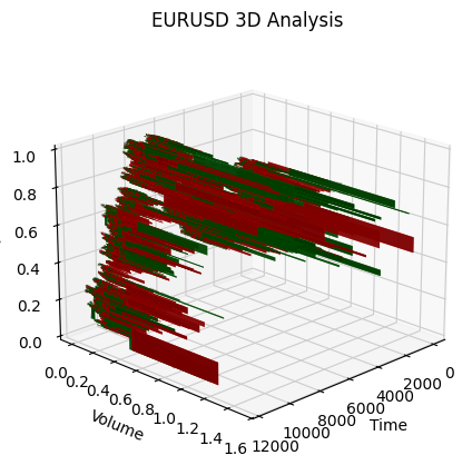
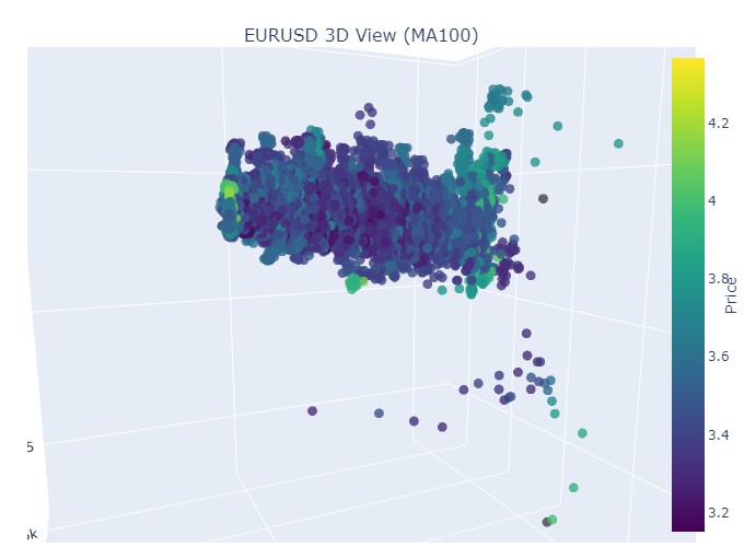
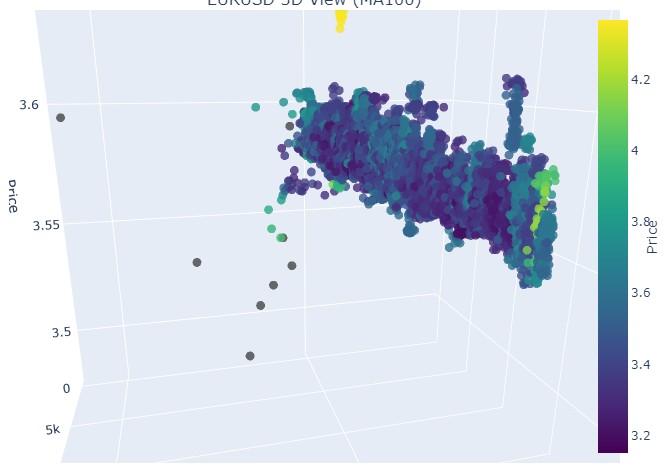
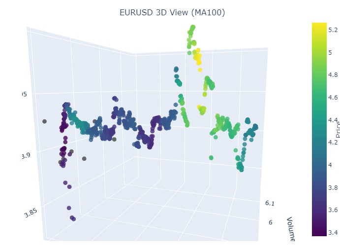
我们选取第一段数据——EURUSD，时间从 2017 年 1 月 1 日到 2018 年 2 月 1 日。实际上，这是一段非常强劲的看涨趋势。准备好看看它在 3D 柱状图中的样子了吗？

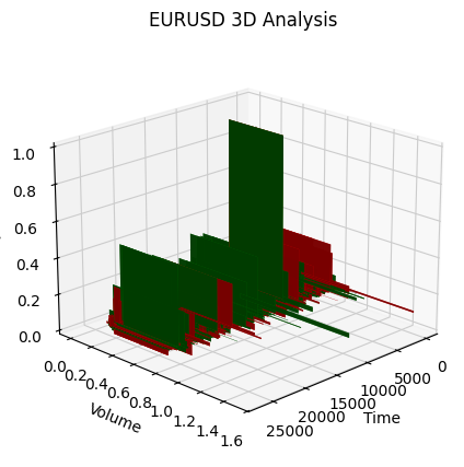
这是另一种可视化的样子：

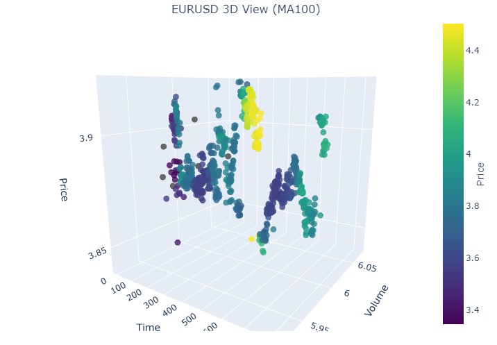
我们来看上升趋势的开始部分：

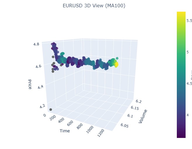
以及它的结束部分：

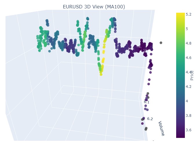
现在我们来看下降趋势。时间从 2018 年 2 月 1 日到 2020 年 3 月 20 日：

这是看跌趋势的开始：

以及它的结束：

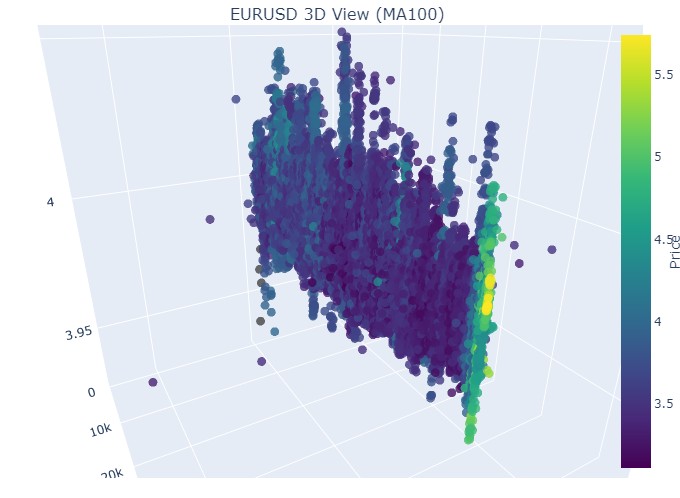
因此我们看到，在 3D 表现中，两种趋势（无论看涨还是看跌）都始于 3D 点密度下方的点区域。而两种情况下趋势的结束，都以明亮的黄色配色为标志。 

为了描述这一现象，以及 EURUSD 在看涨和看跌趋势中的价格行为，可以使用以下通用方程：

P(t) = P_0 + \int_{t_0}^{t} A \cdot e^{k(t-u)} \cdot V(u) \, du + N(t)

其中：

•  P(t) — 某一时刻的货币价格。
•  P_0 — 某一时刻的初始价格。
•  A — 趋势振幅，表征价格变化的规模。
•  k — 决定变化速率的比率（k > 0 表示看涨趋势；k < 0 表示看跌趋势）。
•  V(u) — 给定时间的交易量，影响市场活动，并可能增强价格变化的重要性。
•  N(t) — 随机噪声，反映不可预测的市场波动。

文字解释

该方程描述了货币价格如何随时间变化，取决于多种因素。初始价格是起点，之后积分部分考虑了趋势振幅及其变化速率的影响，使价格根据幅度呈指数增长或下降。由函数 V(u) 表示的交易量增加了另一个维度，表明市场活动也会影响价格变化。

因此，该模型允许可视化不同趋势下的价格走势，将其展示在 3D 空间中，时间轴、价格和成交量共同构建出市场活动的丰富图景。此模式中配色方案的亮度可指示趋势的强度，较亮的颜色对应较高的价格导数和交易量值，预示着市场中强烈的成交量变动。

显示反转

我们来看 11 月 14 日至 11 月 28 日的这段时间。报价反转大约发生在这段时间的中间。这在 3D 坐标中是什么样子？如下所示：

我们在反转时刻和归一化价格坐标上升时看到了熟悉的黄色。现在我们再看另一段带有趋势反转的价格区间，从 2024 年 9 月 13 日到同年 10 月 10 日：

我们再次看到同样的画面，只是黄色及其累积现在出现在底部。看起来很有趣。  

2024 年 8 月 19 日至 8 月 30 日，在此日期范围中间可以看到趋势的精确反转。我们来看看我们的坐标。

再次，完全相同的画面。我们来看 2024 年 7 月 17 日至 8 月 8 日的这段时间。模型会显示出即将反转的迹象吗？

最后一段是 2023 年 4 月 21 日至 8 月 10 日。看涨趋势在那里结束。

我们再次看到了熟悉的黄色。

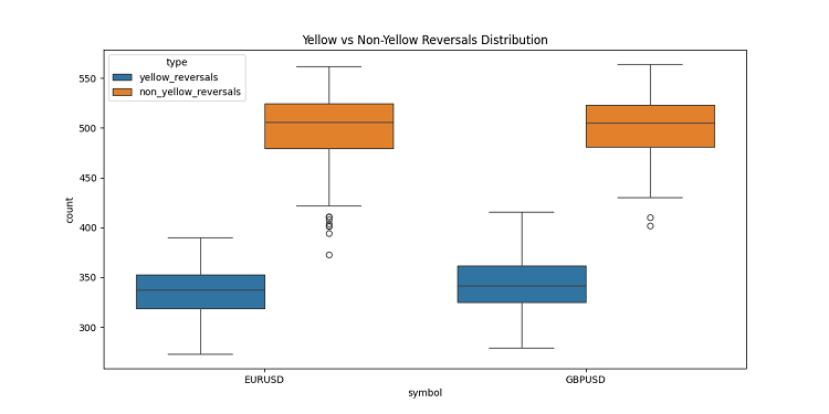
黄色聚类

在开发 3D 柱状图的过程中，我发现了一个非常有趣的特征——黄色成交量-波动率聚类。它们在图表上的行为让我着迷！在查阅了大量历史数据后（准确地说，是 2022-2024 年超过 40 万根柱状图），我注意到了一些令人惊讶的现象。

起初我简直不敢相信自己的眼睛——在大约 10 万根黄色柱状图中，几乎全部（97%！）都出现在价格反转附近。而且，这一现象在正负三根柱状图的范围内都成立。有趣的是，只有 40% 的反转（总共约有 16.9 万次）显示了黄色柱状图。由此可见，黄色柱状图几乎可以保证反转，尽管反转也可能在没有它们的情况下发生。

进一步深入研究趋势后，我注意到了一个清晰的规律。在趋势的开始和持续期间，几乎没有黄色柱状图，只有密集排列的普通 3D 柱状图。但在反转之前，黄色聚类便会在图表上闪耀。

在长期趋势中这一点尤其明显。例如，EURUSD 从 2017 年初上涨至 2018 年 2 月，然后下跌至 2020 年 3 月。在这两种情况下，这些黄色聚类都在反转前出现，它们在 3D 空间中的位置几乎就预示了价格将走向何方！

我也在短期时间段上测试了这一点——我选取了 2024 年中的几个 2-3 周的片段。它就像钟表一样精准！每次在反转之前，黄色柱状图都会出现，仿佛在警告：“嘿，伙计，趋势要反转了！”

这不仅仅是一个指标。我认为，我们触及了市场结构中真正重要的东西——即成交量的分布方式，以及趋势变化前波动率的变化方式。现在当我在 3D 图表上看到黄色聚类时，我就知道是时候为反转做准备了！

结论

在我们结束对 3D 柱状图的探索时，我不得不感叹，这次深入探索多么深刻地改变了我对市场微观结构的理解。最初只是一次可视化实验，后来演变成了一种看待和理解市场的全新方式。

在进行这个项目的过程中，我不断意识到，我们被传统的二维价格表示方式限制得多么严重。转向三维分析为理解价格、成交量和时间之间的关系开辟了全新的视野。尤其令我震惊的是，在三维空间中，重要市场事件之前的模式显现得如此清晰。

最重要的发现是能够及早发现潜在的趋势反转。3D图形中成交量的特征性累积和颜色的变化，已被证明是即将到来的趋势变化的可靠指标。这不仅仅是理论观察——我们已通过大量历史实例验证了这一点。

我们开发的数学模型不仅使我们能够可视化，还能定量评估市场动态。现代可视化技术和软件工具的集成，使得该方法能够应用于实际交易中。我每天都在使用这些工具，它们对我的市场分析方法产生了巨大影响。

然而，我相信我们才刚刚起步。这个项目打开了多元市场微观结构分析的大门，我坚信，在这一方向上的进一步研究将带来更多有趣的发现。也许，下一步将是整合机器学习来自动识别 3D 模式，或基于多元分析开发新的交易策略。

最终，这项研究的真正价值不在于漂亮的图表或复杂的方程，而在于它所提供的对市场的全新认知。作为一名研究者，我坚信技术分析的未来在于对市场数据的多元分析方法。