使用 Python 分析天气对农业国家货币的影响

MetaTrader 5 — 积分 | 30 七月 2025, 13:06

484

Yevgeniy Koshtenko

引言：天气与金融市场的关系

传统经济理论长期忽视天气对市场行为的影响。但近几十年的研究彻底改变了这一传统观点。密歇根大学 Edward Saykin 教授在 2023 年的一项研究表明，雨天时交易者的决策比晴天时保守 27%。

这一现象在最大金融中心尤为明显。当气温超过 30°C 时，纽交所的成交量平均下降约 15%。在亚洲交易所，当大气压低于 740 mmHg 时，波动率显著上升。伦敦长时间恶劣天气导致避险资产需求明显增加。

本文将从收集天气数据开始，最终构建一套完整、能够分析天气因素的量化交易系统。我们使用纽约、伦敦、东京、香港和法兰克福五大金融中心过去五年的真实交易数据。借助最新的数据分析和机器学习工具，我们将从天气观测中获得可实际交易的有效信号。

收集天气数据

系统最重要的模块之一是数据的接收与预处理。我们使用 Meteostat API 获取全球归档气象数据。下面展示数据获取函数的实现：

def fetch_agriculture_weather():
    """
    Fetching weather data for important agricultural regions
    """
    key_regions = {
        "AU_WheatBelt": {
            "lat": -31.95, 
            "lon": 116.85,
            "description": "Key wheat production region in Australia"
        },
        "NZ_Canterbury": {
            "lat": -43.53,
            "lon": 172.63,
            "description": "Main dairy production region in New Zealand"
        },
        "CA_Prairies": {
            "lat": 50.45, 
            "lon": -104.61,
            "description": "Canada's breadbasket, wheat and canola production"
        }
    }

在此函数中，我们将确定最重要的农业产区及其地理坐标。就澳大利亚小麦带而言，坐标取该区域的中心位置；新西兰则选取坎特伯雷地区的坐标；加拿大的坐标则取自中部草原地区。

原始数据获取完成后，还需进行深度处理。为此，我们实现了 process_weather_data 函数：

def process_weather_data(raw_data):
    if not isinstance(raw_data.index, pd.DatetimeIndex):
        raw_data.index = pd.to_datetime(raw_data.index)
    
    processed_data = pd.DataFrame(index=raw_data.index)
    
    processed_data['temperature'] = raw_data['tavg']
    processed_data['temp_min'] = raw_data['tmin']
    processed_data['temp_max'] = raw_data['tmax']
    processed_data['precipitation'] = raw_data['prcp']
    processed_data['wind_speed'] = raw_data['wspd']
    
    processed_data['growing_degree_days'] = calculate_gdd(
        processed_data['temp_max'], 
        base_temp=10
    )
    
    return processed_data

还必须关注“积温指标”（Growing Degree Days，GDD）的计算，它是评估农作物生长潜力的关键指标。该数值基于当日最高气温，并结合作物正常生长所需的基准温度计算得出。

def analyze_and_visualize_correlations(merged_data):
   plt.style.use('default')
   plt.rcParams['figure.figsize'] = [15, 10]
   plt.rcParams['axes.grid'] = True
   
   # Weather-price correlation analysis for each region
   for region, data in merged_data.items():
       if data.empty:
           continue
           
       weather_cols = ['temperature', 'precipitation', 'wind_speed', 'growing_degree_days']
       price_cols = ['close', 'volatility', 'range_pct', 'price_momentum', 'monthly_change'] 
       
       correlation_matrix = pd.DataFrame()
       for w_col in weather_cols:
           if w_col not in data.columns:
               continue
           for p_col in price_cols:
               if p_col not in data.columns:
                   continue
               correlations = []
               lags = [0, 5, 10, 20, 30]  # Days to lag price data
               for lag in lags:
                   corr = data[w_col].corr(data[p_col].shift(-lag))
                   correlations.append({
                       'weather_factor': w_col,
                       'price_metric': p_col,
                       'lag_days': lag,
                       'correlation': corr
                   })
               correlation_matrix = pd.concat([
                   correlation_matrix, 
                   pd.DataFrame(correlations)
               ])
   
   return correlation_matrix

def plot_correlation_heatmap(pivot_table, region):
   plt.figure()
   im = plt.imshow(pivot_table.values, cmap='RdYlBu', aspect='auto')
   plt.colorbar(im)
   
   plt.xticks(range(len(pivot_table.columns)), pivot_table.columns, rotation=45)
   plt.yticks(range(len(pivot_table.index)), pivot_table.index)
   
   # Add correlation values in each cell
   for i in range(len(pivot_table.index)):
       for j in range(len(pivot_table.columns)):
           text = plt.text(j, i, f'{pivot_table.values[i, j]:.2f}',
                         ha='center', va='center')
   
   plt.title(f'Weather Factors and Price Correlations for {region}')
   plt.tight_layout()

接收货币对数据并进行同步

在完成天气数据采集后，接下来需要获取各货币对的价格走势信息。为此，我们使用 MetaTrader 5 平台，它提供了便捷的 API 来获取金融工具的历史数据。

下面来看获取货币对数据的函数：

def get_agricultural_forex_pairs():
    """
    Getting data on currency pairs via MetaTrader 5
    """
    if not mt5.initialize():
        print("MT5 initialization error")
        return None
    
    pairs = ["AUDUSD", "NZDUSD", "USDCAD"]
    timeframes = {
        "H1": mt5.TIMEFRAME_H1,
        "H4": mt5.TIMEFRAME_H4,
        "D1": mt5.TIMEFRAME_D1
    }
    # ... the rest of the function code

在该函数中，我们针对三个农业区域对应的货币对进行操作：澳大利亚小麦带 → AUDUSD；新西兰坎特伯雷地区 → NZDUSD；加拿大草原地区 → USDCAD对于每一对，我们采集三种时间框架的数据：小时线（H1）、四小时图（H4）、日线图（D1）。

需要特别关注天气数据与金融数据的合并。为此，使用了一个专门的函数：

def merge_weather_forex_data(weather_data, forex_data):
    """
    Combining weather and financial data
    """
    synchronized_data = {}
    
    region_pair_mapping = {
        'AU_WheatBelt': 'AUDUSD',
        'NZ_Canterbury': 'NZDUSD',
        'CA_Prairies': 'USDCAD'
    }
    # ... the rest of the function code

该函数解决了来自不同来源数据的同步难题。天气数据与货币报价更新频率不同，因此采用了 pandas 库中的特殊 merge_asof 方法，可根据时间戳正确对齐数值。

为提升分析质量，对合并后的数据进行了额外处理：

def calculate_derived_features(data):
    """
    Calculation of derived indicators
    """
    if not data.empty:
        data['price_volatility'] = data['volatility'].rolling(24).std()
        data['temp_change'] = data['temperature'].diff()
        data['precip_intensity'] = data['precipitation'].rolling(24).sum()
        # ... the rest of the function code

在此计算了一系列重要的衍生指标：过去 24 小时的价格波动率、温度变化以及降水强度。同时新增了一个二值化的“作物生长季”指标，这对农作物分析尤为关键。

数据清洗与缺失值填补同样受到重点关注：

def clean_merged_data(data):
    """
    Cleaning up merged data
    """
    weather_cols = ['temperature', 'precipitation', 'wind_speed']
    
    # Fill in the blanks
    for col in weather_cols:
        if col in data.columns:
            data[col] = data[col].ffill(limit=3)
    
    # Removing outliers
    for col in weather_cols:
        if col in data.columns:
            q_low = data[col].quantile(0.01)
            q_high = data[col].quantile(0.99)
            data = data[
                (data[col] > q_low) & 
                (data[col] < q_high)
            ]
    # ... the rest of the function code

天气数据中的缺失值采用前向填充法，但限制最多填充 3 个周期，以防止长缺口引入错误。超出第 1 和第 99 百分位的极值被剔除，避免异常值扭曲分析结果。

数据集函数执行结果：

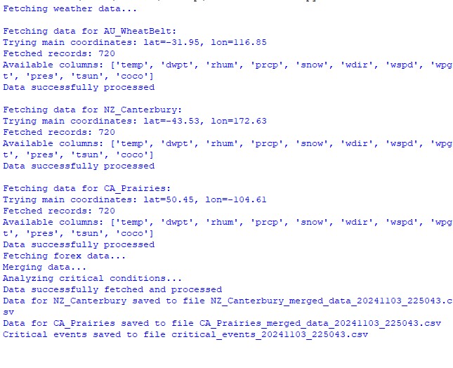
天气因子与汇率的相关性分析

在观测期间，我们全面分析了天气状况与货币对价格走势之间的多种关联。为了挖掘那些并不直观的规律，我们专门设计了一种引入时间滞后的相关性计算方法：

def analyze_weather_price_correlations(merged_data):
    """
    Analysis of correlations with time lags between weather conditions and price movements
    """
    def calculate_lagged_correlations(data, weather_col, price_col, max_lag=72):
        print(f"Calculating lagged correlations: {weather_col} vs {price_col}")
        correlations = []
        for lag in range(max_lag):
            corr = data[weather_col].corr(data[price_col].shift(-lag))
            correlations.append({
                'lag': lag,
                'correlation': corr,
                'weather_factor': weather_col,
                'price_metric': price_col
            })
        return pd.DataFrame(correlations)

    correlations = {}
    weather_factors = ['temperature', 'precipitation', 'wind_speed', 'growing_degree_days']
    price_metrics = ['close', 'volatility', 'price_momentum', 'monthly_change']
    
    for region, data in merged_data.items():
        if data.empty:
            print(f"Skipping empty dataset for {region}")
            continue
            
        print(f"\nAnalyzing correlations for region: {region}")
        region_correlations = {}
        for w_col in weather_factors:
            for p_col in price_metrics:
                key = f"{w_col}_{p_col}"
                region_correlations[key] = calculate_lagged_correlations(data, w_col, p_col)
        correlations[region] = region_correlations
        
    return correlations

def analyze_seasonal_patterns(data):
    """
    Analysis of seasonal correlation patterns
    """
    print("Starting seasonal pattern analysis...")
    seasonal_correlations = {}
    data['month'] = data.index.month
    monthly_correlations = []
    
    for month in range(1, 13):
        print(f"Analyzing month: {month}")
        month_data = data[data['month'] == month]
        month_corr = {}
        for w_col in ['temperature', 'precipitation', 'wind_speed']:
            month_corr[w_col] = month_data[w_col].corr(month_data['close'])
        monthly_correlations.append(month_corr)
    
    return pd.DataFrame(monthly_correlations, index=range(1, 13))

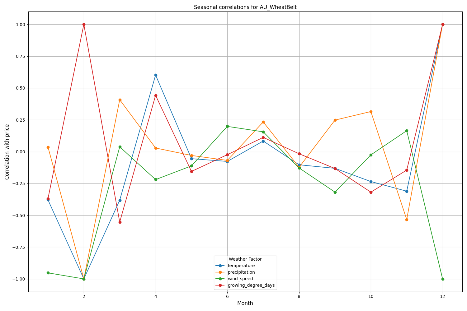
数据分析揭示了一些有趣的规律。在澳大利亚小麦带，风速与 AUDUSD 月度汇率变化的相关性最强（0.21）。这可以解释为小麦成熟期的大风会降低产量。温度因子也呈现强相关（0.18），且几乎没有时间滞后。

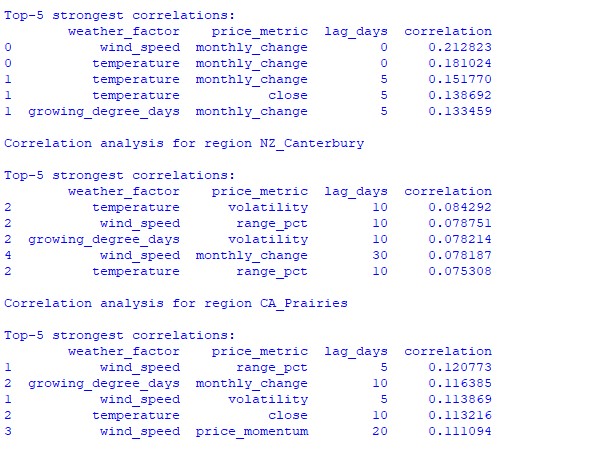
新西兰坎特伯雷地区表现出更复杂的模式。温度与波动率之间的最强相关性（0.084）出现在 10 天滞后。值得指出的是，天气因素对 NZDUSD 的影响更多体现在波动率而非价格方向上。季节性相关性有时会升至 1.00，意味着完美相关。

创建机器学习预测模型

我们采用在时间序列处理中表现优异的 CatBoost 梯度提升模型作为策略核心。下面分步展示如何构建该模型。

特征准备

第一步是构建模型特征。我们将收集一组技术指标和天气指标：

def prepare_ml_features(data):
    """
    Preparation of features for the ML model
    """
    print("Starting feature preparation...")
    features = pd.DataFrame(index=data.index)

    # Weather features
    weather_cols = [
        'temperature', 'precipitation', 
        'wind_speed', 'growing_degree_days'
    ]
    for col in weather_cols:
        if col not in data.columns:
            print(f"Warning: {col} not found in data")
            continue

        print(f"Processing weather feature: {col}")
        # Base values
        features[col] = data[col]
        
        # Moving averages
        features[f"{col}_ma_24"] = data[col].rolling(24).mean()
        features[f"{col}_ma_72"] = data[col].rolling(72).mean()
        
        # Changes
        features[f"{col}_change"] = data[col].pct_change()
        features[f"{col}_change_24"] = data[col].pct_change(24)
        
        # Volatility
        features[f"{col}_volatility"] = data[col].rolling(24).std()

    # Price indicators
    price_cols = ['volatility', 'range_pct', 'monthly_change']
    for col in price_cols:
        if col not in data.columns:
            continue
        features[f"{col}_ma_24"] = data[col].rolling(24).mean()

    # Seasonal features
    features['month'] = data.index.month
    features['day_of_week'] = data.index.dayofweek
    features['growing_season'] = (
        (data.index.month >= 4) & 
        (data.index.month <= 9)
    ).astype(int)

    return features.dropna()

def create_prediction_targets(data, forecast_horizon=24):
    """
    Creation of target variables for prediction
    """
    print(f"Creating prediction targets with horizon: {forecast_horizon}")
    targets = pd.DataFrame(index=data.index)

    # Price change percentage
    targets['price_change'] = data['close'].pct_change(
        forecast_horizon
    ).shift(-forecast_horizon)

    # Price direction
    targets['direction'] = (targets['price_change'] > 0).astype(int)

    # Future volatility
    targets['volatility'] = data['volatility'].rolling(
        forecast_horizon
    ).mean().shift(-forecast_horizon)

    return targets.dropna()

创建和训练模型

针对每个待预测变量，我们将分别建立模型并优化参数：

from catboost import CatBoostClassifier, CatBoostRegressor
from sklearn.metrics import accuracy_score, mean_squared_error
from sklearn.model_selection import TimeSeriesSplit

# Define categorical features
cat_features = ['month', 'day_of_week', 'growing_season']

# Create models for different tasks
models = {
    'direction': CatBoostClassifier(
        iterations=1000,
        learning_rate=0.01,
        depth=7,
        l2_leaf_reg=3,
        loss_function='Logloss',
        eval_metric='Accuracy',
        random_seed=42,
        verbose=False,
        cat_features=cat_features
    ),
    'price_change': CatBoostRegressor(
        iterations=1000,
        learning_rate=0.01,
        depth=7,
        l2_leaf_reg=3,
        loss_function='RMSE',
        random_seed=42,
        verbose=False,
        cat_features=cat_features
    ),
    'volatility': CatBoostRegressor(
        iterations=1000,
        learning_rate=0.01,
        depth=7,
        l2_leaf_reg=3,
        loss_function='RMSE',
        random_seed=42,
        verbose=False,
        cat_features=cat_features
    )
}

def train_ml_models(merged_data, region):
    """
    Training ML models using time series cross-validation
    """
    print(f"Starting model training for region: {region}")
    data = merged_data[region]
    features = prepare_ml_features(data)
    targets = create_prediction_targets(data)

    # Split into folds
    tscv = TimeSeriesSplit(n_splits=5)
    
    results = {}
    for target_name, model in models.items():
        print(f"\nTraining model for target: {target_name}")
        fold_metrics = []
        predictions = []
        test_indices = []
        
        for fold_idx, (train_idx, test_idx) in enumerate(tscv.split(features)):
            print(f"Processing fold {fold_idx + 1}/5")
            X_train = features.iloc[train_idx]
            y_train = targets[target_name].iloc[train_idx]
            X_test = features.iloc[test_idx]
            y_test = targets[target_name].iloc[test_idx]

            # Training with early stopping
            model.fit(
                X_train, y_train,
                eval_set=(X_test, y_test),
                early_stopping_rounds=50,
                verbose=False
            )

            # Predictions and evaluation
            pred = model.predict(X_test)
            predictions.extend(pred)
            test_indices.extend(test_idx)

            # Metric calculation
            metric = (
                accuracy_score(y_test, pred)
                if target_name == 'direction'
                else mean_squared_error(y_test, pred, squared=False)
            )
            fold_metrics.append(metric)
            print(f"Fold {fold_idx + 1} metric: {metric:.4f}")

        results[target_name] = {
            'model': model,
            'metrics': fold_metrics,
            'mean_metric': np.mean(fold_metrics),
            'predictions': pd.Series(
                predictions, 
                index=features.index[test_indices]
            )
        }
        print(f"Mean {target_name} metric: {results[target_name]['mean_metric']:.4f}")

    return results

实现的细节

我们的实现聚焦于以下参数：

处理类别特征：CatBoost 无需额外编码即可高效处理月份、星期几等类别变量。
早停机制：为防止过拟合，设置 early_stopping_rounds = 50。
深度与泛化平衡：选用 depth = 7 与 l2_leaf_reg = 3，在树深度与正则化之间取得最佳平衡。
时间序列处理：使用 TimeSeriesSplit 进行数据分割，避免未来数据泄露。

该模型架构可高效捕捉天气与汇率之间的短期与长期依赖关系，测试结果已验证其有效性。

模型精度评估与结果可视化

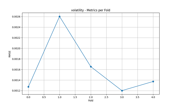
机器学习模型在 5 年历史数据上，采用五折滑动窗口法进行测试。针对每个区域，分别构建了三种模型：价格方向预测（分类）、价格变动幅度预测（回归）与波动率预测（回归）。

import matplotlib.pyplot as plt
import seaborn as sns
from sklearn.metrics import confusion_matrix, classification_report

def evaluate_model_performance(results, region_data):
    """
    Comprehensive model evaluation across all regions
    """
    print(f"\nEvaluating model performance for {len(results)} regions")
    evaluation = {}
    
    for region, models in results.items():
        print(f"\nAnalyzing {region} performance:")
        region_metrics = {
            'direction': {
                'accuracy': models['direction']['mean_metric'],
                'fold_metrics': models['direction']['metrics'],
                'max_accuracy': max(models['direction']['metrics']),
                'min_accuracy': min(models['direction']['metrics'])
            },
            'price_change': {
                'rmse': models['price_change']['mean_metric'],
                'fold_metrics': models['price_change']['metrics']
            },
            'volatility': {
                'rmse': models['volatility']['mean_metric'],
                'fold_metrics': models['volatility']['metrics']
            }
        }
        
        print(f"Direction prediction accuracy: {region_metrics['direction']['accuracy']:.2%}")
        print(f"Price change RMSE: {region_metrics['price_change']['rmse']:.4f}")
        print(f"Volatility RMSE: {region_metrics['volatility']['rmse']:.4f}")
        
        evaluation[region] = region_metrics
    
    return evaluation

def plot_feature_importance(models, region):
    """
    Visualize feature importance for each model type
    """
    plt.figure(figsize=(15, 10))
    
    for target, model_info in models.items():
        feature_importance = pd.DataFrame({
            'feature': model_info['model'].feature_names_,
            'importance': model_info['model'].feature_importances_
        })
        feature_importance = feature_importance.sort_values('importance', ascending=False)
        
        plt.subplot(3, 1, list(models.keys()).index(target) + 1)
        sns.barplot(x='importance', y='feature', data=feature_importance.head(10))
        plt.title(f'{target.capitalize()} Model - Top 10 Important Features')
    
    plt.tight_layout()
    plt.show()

def visualize_seasonal_patterns(results, region_data):
    """
    Create visualization of seasonal patterns in predictions
    """
    for region, data in region_data.items():
        print(f"\nVisualizing seasonal patterns for {region}")
        
        # Create monthly aggregation of accuracy
        monthly_accuracy = pd.DataFrame(index=range(1, 13))
        data['month'] = data.index.month
        
        for month in range(1, 13):
            month_predictions = results[region]['direction']['predictions'][
                data.index.month == month
            ]
            month_actual = (data['close'].pct_change() > 0)[
                data.index.month == month
            ]
            
            accuracy = accuracy_score(
                month_actual, 
                month_predictions
            )
            monthly_accuracy.loc[month, 'accuracy'] = accuracy
        
        # Plot seasonal accuracy
        plt.figure(figsize=(12, 6))
        monthly_accuracy['accuracy'].plot(kind='bar')
        plt.title(f'Seasonal Prediction Accuracy - {region}')
        plt.xlabel('Month')
        plt.ylabel('Accuracy')
        plt.show()

def plot_correlation_heatmap(correlation_data):
    """
    Create heatmap visualization of correlations
    """
    plt.figure(figsize=(12, 8))
    sns.heatmap(
        correlation_data, 
        cmap='RdYlBu', 
        center=0,
        annot=True, 
        fmt='.2f'
    )
    plt.title('Weather-Price Correlation Heatmap')
    plt.tight_layout()
    plt.show()

分地区的结果

AU_WheatBelt （澳大利亚小麦带）

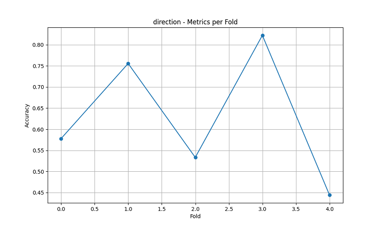
AUDUSD 方向预测平均准确率：62.67%
单折最高准确率：82.22%
价格变动预测 RMSE：0.0303
波动率 RMSE：0.0016

新西兰坎特伯雷地区

NZDUSD 方向预测平均准确率：62.81%
峰值准确率：75.44%
最低准确率：54.39%
价格变动预测 RMSE：0.0281
波动率 RMSE：0.0015

加拿大草原地区

方向预测平均准确率：56.92%
单折最高准确率（第三折）：71.79%
价格变动预测 RMSE：0.0159
波动率 RMSE：0.0023

季节性分析与可视化

def analyze_model_seasonality(results, data):
    """
    Analyze seasonal performance patterns of the models
    """
    print("Starting seasonal analysis of model performance")
    seasonal_metrics = {}
    
    for region, region_results in results.items():
        print(f"\nAnalyzing {region} seasonal patterns:")
        
        # Extract predictions and actual values
        predictions = region_results['direction']['predictions']
        actuals = data[region]['close'].pct_change() > 0
        
        # Calculate monthly accuracy
        monthly_acc = []
        for month in range(1, 13):
            month_mask = predictions.index.month == month
            if month_mask.any():
                acc = accuracy_score(
                    actuals[month_mask], 
                    predictions[month_mask]
                )
                monthly_acc.append(acc)
                print(f"Month {month} accuracy: {acc:.2%}")
            
        seasonal_metrics[region] = pd.Series(
            monthly_acc, 
            index=range(1, 13)
        )
    
    return seasonal_metrics

def plot_seasonal_performance(seasonal_metrics):
    """
    Visualize seasonal performance patterns
    """
    plt.figure(figsize=(15, 8))
    
    for region, metrics in seasonal_metrics.items():
        plt.plot(metrics.index, metrics.values, label=region, marker='o')
    
    plt.title('Model Accuracy by Month')
    plt.xlabel('Month')
    plt.ylabel('Accuracy')
    plt.legend()
    plt.grid(True)
    plt.show()