Pythonによる農業国通貨への天候影響分析

はじめに：天候と金融市場の関係

古典的な経済理論は、天候のような要因が市場の動きに与える影響を長い間無視してきました。しかし、ここ数十年の研究によって、その従来の見方は完全に変わりました。ミシガン大学のEdward Saykin教授が2023年におこなった研究では、雨の日にはトレーダーの意思決定が晴れの日と比べて27%慎重になることが示されました。

これは特に、世界の主要な金融センターで顕著に見られます。気温が30℃を超える日には、ニューヨーク証券取引所での取引量が平均して約15%減少します。アジアの取引所では、気圧が740 mmHgを下回ると、ボラティリティが高まる傾向があります。ロンドンでは悪天候が長期間続くと、安全資産への需要が明らかに増加します。

本記事では、まず天候データの収集から始め、天候要因を分析する完全な取引システムの構築へと進んでいきます。私たちの作業は、ニューヨーク、ロンドン、東京、香港、フランクフルトといった世界の主要金融センターにおける過去5年間の実際の取引データに基づいています。最新のデータ分析および機械学習ツールを用いて、天候観測から実際の取引シグナルを導き出します。

気象データの収集

システムにおける最も重要な要素の一つは、データの取得および前処理をおこなうモジュールです。気象データを扱うために、私たちは世界中の過去の気象データにアクセスできるMeteostat APIを使用します。それでは、データ取得関数がどのように実装されているかを見てみましょう。

def fetch_agriculture_weather():
    """
    Fetching weather data for important agricultural regions
    """
    key_regions = {
        "AU_WheatBelt": {
            "lat": -31.95, 
            "lon": 116.85,
            "description": "Key wheat production region in Australia"
        },
        "NZ_Canterbury": {
            "lat": -43.53,
            "lon": 172.63,
            "description": "Main dairy production region in New Zealand"
        },
        "CA_Prairies": {
            "lat": 50.45, 
            "lon": -104.61,
            "description": "Canada's breadbasket, wheat and canola production"
        }
    }

この関数では、最も重要な農業地域とその位置座標を特定します。オーストラリアの「小麦ベルト」については、地域の中央部の座標を使用します。ニュージーランドについては、カンタベリー地方の座標を、カナダについては、プレーリー地域の中央部の座標をそれぞれ使用します。

生データを取得した後には、本格的な処理が必要になります。そのために、process_weather_data関数が実装されています。

def process_weather_data(raw_data):
    if not isinstance(raw_data.index, pd.DatetimeIndex):
        raw_data.index = pd.to_datetime(raw_data.index)
    
    processed_data = pd.DataFrame(index=raw_data.index)
    
    processed_data['temperature'] = raw_data['tavg']
    processed_data['temp_min'] = raw_data['tmin']
    processed_data['temp_max'] = raw_data['tmax']
    processed_data['precipitation'] = raw_data['prcp']
    processed_data['wind_speed'] = raw_data['wspd']
    
    processed_data['growing_degree_days'] = calculate_gdd(
        processed_data['temp_max'], 
        base_temp=10
    )
    
    return processed_data

農作物の成長ポテンシャルを評価するために必要な指標である生育日数(GDD: Growing Degree Days)の計算にも注意を払う必要があります。この指標は、植物の通常の生育温度を考慮しながら、日中の最高気温に基づいて算出されます。

def analyze_and_visualize_correlations(merged_data):
   plt.style.use('default')
   plt.rcParams['figure.figsize'] = [15, 10]
   plt.rcParams['axes.grid'] = True
   
   # Weather-price correlation analysis for each region
   for region, data in merged_data.items():
       if data.empty:
           continue
           
       weather_cols = ['temperature', 'precipitation', 'wind_speed', 'growing_degree_days']
       price_cols = ['close', 'volatility', 'range_pct', 'price_momentum', 'monthly_change'] 
       
       correlation_matrix = pd.DataFrame()
       for w_col in weather_cols:
           if w_col not in data.columns:
               continue
           for p_col in price_cols:
               if p_col not in data.columns:
                   continue
               correlations = []
               lags = [0, 5, 10, 20, 30]  # Days to lag price data
               for lag in lags:
                   corr = data[w_col].corr(data[p_col].shift(-lag))
                   correlations.append({
                       'weather_factor': w_col,
                       'price_metric': p_col,
                       'lag_days': lag,
                       'correlation': corr
                   })
               correlation_matrix = pd.concat([
                   correlation_matrix, 
                   pd.DataFrame(correlations)
               ])
   
   return correlation_matrix

def plot_correlation_heatmap(pivot_table, region):
   plt.figure()
   im = plt.imshow(pivot_table.values, cmap='RdYlBu', aspect='auto')
   plt.colorbar(im)
   
   plt.xticks(range(len(pivot_table.columns)), pivot_table.columns, rotation=45)
   plt.yticks(range(len(pivot_table.index)), pivot_table.index)
   
   # Add correlation values in each cell
   for i in range(len(pivot_table.index)):
       for j in range(len(pivot_table.columns)):
           text = plt.text(j, i, f'{pivot_table.values[i, j]:.2f}',
                         ha='center', va='center')
   
   plt.title(f'Weather Factors and Price Correlations for {region}')
   plt.tight_layout()

通貨ペアのデータ取得と同期

天候データの収集を設定した後は、通貨ペアの動きに関する情報を取得する処理を実装する必要があります。これを実現するために、金融商品の過去データを扱う便利なAPIを提供しているMetaTrader 5プラットフォームを使用します。

それでは、通貨ペアのデータを取得する関数について見ていきましょう。

def get_agricultural_forex_pairs():
    """
    Getting data on currency pairs via MetaTrader 5
    """
    if not mt5.initialize():
        print("MT5 initialization error")
        return None
    
    pairs = ["AUDUSD", "NZDUSD", "USDCAD"]
    timeframes = {
        "H1": mt5.TIMEFRAME_H1,
        "H4": mt5.TIMEFRAME_H4,
        "D1": mt5.TIMEFRAME_D1
    }
    # ... the rest of the function code

この関数では、農業地域に関連する3つの主要な通貨ペアを対象としています。オーストラリアの小麦ベルトにはAUDUSD、カンタベリー地方にはNZDUSD、カナダのプレーリー地域にはUSDCADです。各通貨ペアについて、1時間足(H1)、4時間足(H4)、および日足(D1)の3つの時間軸でデータを収集します。

特に重要なのは、天候データと金融データを統合することです。この役割を担うのが、専用の関数です。

def merge_weather_forex_data(weather_data, forex_data):
    """
    Combining weather and financial data
    """
    synchronized_data = {}
    
    region_pair_mapping = {
        'AU_WheatBelt': 'AUDUSD',
        'NZ_Canterbury': 'NZDUSD',
        'CA_Prairies': 'USDCAD'
    }
    # ... the rest of the function code

この関数は、異なるソースからのデータを同期させるという複雑な問題を解決します。天候データと通貨のレートは更新頻度が異なるため、pandasライブラリの特別なメソッドであるmerge_asofを使用します。これにより、タイムスタンプを考慮して正確に値を比較することが可能になります。

分析の質を向上させるために、結合したデータに対して追加の処理もおこなわれます。

def calculate_derived_features(data):
    """
    Calculation of derived indicators
    """
    if not data.empty:
        data['price_volatility'] = data['volatility'].rolling(24).std()
        data['temp_change'] = data['temperature'].diff()
        data['precip_intensity'] = data['precipitation'].rolling(24).sum()
        # ... the rest of the function code

ここでは、過去24時間の価格変動率、気温の変化、降水量の強さといった重要な派生指標が計算されます。また、農作物の分析に特に重要な「生育期」を示す二値指標も追加されます。

特に、外れ値の除去や欠損値の補完といったデータのクレンジングに重点が置かれています。

def clean_merged_data(data):
    """
    Cleaning up merged data
    """
    weather_cols = ['temperature', 'precipitation', 'wind_speed']
    
    # Fill in the blanks
    for col in weather_cols:
        if col in data.columns:
            data[col] = data[col].ffill(limit=3)
    
    # Removing outliers
    for col in weather_cols:
        if col in data.columns:
            q_low = data[col].quantile(0.01)
            q_high = data[col].quantile(0.99)
            data = data[
                (data[col] > q_low) & 
                (data[col] < q_high)
            ]
    # ... the rest of the function code

この関数では、天候データの欠損値処理に前方補填法を使用していますが、長期間のギャップで誤った値が入るのを防ぐため、3期間までの制限を設けています。また、1パーセンタイルおよび99パーセンタイルを超える極端な値も除去しており、これにより外れ値が分析結果を歪めるのを防いでいます。

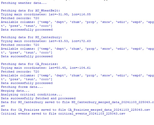
データセット関数の実行結果：

天候要因と価格動向の相関分析

観察期間中、天候条件と通貨ペアの価格変動の関係におけるさまざまな側面が分析されました。すぐには明らかでないパターンを見つけるために、時間遅れを考慮した特別な相関計算手法が作成されました。

def analyze_weather_price_correlations(merged_data):
    """
    Analysis of correlations with time lags between weather conditions and price movements
    """
    def calculate_lagged_correlations(data, weather_col, price_col, max_lag=72):
        print(f"Calculating lagged correlations: {weather_col} vs {price_col}")
        correlations = []
        for lag in range(max_lag):
            corr = data[weather_col].corr(data[price_col].shift(-lag))
            correlations.append({
                'lag': lag,
                'correlation': corr,
                'weather_factor': weather_col,
                'price_metric': price_col
            })
        return pd.DataFrame(correlations)

    correlations = {}
    weather_factors = ['temperature', 'precipitation', 'wind_speed', 'growing_degree_days']
    price_metrics = ['close', 'volatility', 'price_momentum', 'monthly_change']
    
    for region, data in merged_data.items():
        if data.empty:
            print(f"Skipping empty dataset for {region}")
            continue
            
        print(f"\nAnalyzing correlations for region: {region}")
        region_correlations = {}
        for w_col in weather_factors:
            for p_col in price_metrics:
                key = f"{w_col}_{p_col}"
                region_correlations[key] = calculate_lagged_correlations(data, w_col, p_col)
        correlations[region] = region_correlations
        
    return correlations

def analyze_seasonal_patterns(data):
    """
    Analysis of seasonal correlation patterns
    """
    print("Starting seasonal pattern analysis...")
    seasonal_correlations = {}
    data['month'] = data.index.month
    monthly_correlations = []
    
    for month in range(1, 13):
        print(f"Analyzing month: {month}")
        month_data = data[data['month'] == month]
        month_corr = {}
        for w_col in ['temperature', 'precipitation', 'wind_speed']:
            month_corr[w_col] = month_data[w_col].corr(month_data['close'])
        monthly_correlations.append(month_corr)
    
    return pd.DataFrame(monthly_correlations, index=range(1, 13))

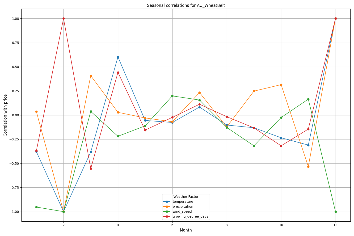
分析の結果、興味深いパターンが明らかになりました。オーストラリアの小麦ベルトにおいて、最も強い相関(0.21)が見られたのは風速とAUDUSD為替レートの月次変動との間でした。これは、小麦の成熟期に強風が収穫量を減少させる可能性があることによって説明できます。また、気温要因も強い相関(0.18)を示しており、ほとんど時間遅れなく影響を及ぼしていることが確認されました。

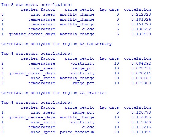
ニュージーランドのカンタベリー地域では、より複雑なパターンが見られます。最も強い相関(0.084)は、気温とボラティリティの間で、10日間の遅れを伴って示されました。また、天候要因がNZDUSDに与える影響は、価格の動きの方向性よりもボラティリティにより強く反映されていることに注意が必要です。季節的な相関が1.00に達することもあり、これは完全な相関を示します。

機械学習モデルの作成と予測

私たちの戦略は、時系列データの取り扱いに優れていることが実証されているCatBoost勾配ブースティングモデルに基づいています。モデルの作成を段階的に見ていきましょう。

特徴量の作成

最初のステップは、モデルの特徴量を形成することです。技術的指標と天候指標の選択を収集していきます。

def prepare_ml_features(data):
    """
    Preparation of features for the ML model
    """
    print("Starting feature preparation...")
    features = pd.DataFrame(index=data.index)

    # Weather features
    weather_cols = [
        'temperature', 'precipitation', 
        'wind_speed', 'growing_degree_days'
    ]
    for col in weather_cols:
        if col not in data.columns:
            print(f"Warning: {col} not found in data")
            continue

        print(f"Processing weather feature: {col}")
        # Base values
        features[col] = data[col]
        
        # Moving averages
        features[f"{col}_ma_24"] = data[col].rolling(24).mean()
        features[f"{col}_ma_72"] = data[col].rolling(72).mean()
        
        # Changes
        features[f"{col}_change"] = data[col].pct_change()
        features[f"{col}_change_24"] = data[col].pct_change(24)
        
        # Volatility
        features[f"{col}_volatility"] = data[col].rolling(24).std()

    # Price indicators
    price_cols = ['volatility', 'range_pct', 'monthly_change']
    for col in price_cols:
        if col not in data.columns:
            continue
        features[f"{col}_ma_24"] = data[col].rolling(24).mean()

    # Seasonal features
    features['month'] = data.index.month
    features['day_of_week'] = data.index.dayofweek
    features['growing_season'] = (
        (data.index.month >= 4) & 
        (data.index.month <= 9)
    ).astype(int)

    return features.dropna()

def create_prediction_targets(data, forecast_horizon=24):
    """
    Creation of target variables for prediction
    """
    print(f"Creating prediction targets with horizon: {forecast_horizon}")
    targets = pd.DataFrame(index=data.index)

    # Price change percentage
    targets['price_change'] = data['close'].pct_change(
        forecast_horizon
    ).shift(-forecast_horizon)

    # Price direction
    targets['direction'] = (targets['price_change'] > 0).astype(int)

    # Future volatility
    targets['volatility'] = data['volatility'].rolling(
        forecast_horizon
    ).mean().shift(-forecast_horizon)

    return targets.dropna()

モデルの作成と学習

検討する各変数について、最適化されたパラメータを持つ個別のモデルを作成します。

from catboost import CatBoostClassifier, CatBoostRegressor
from sklearn.metrics import accuracy_score, mean_squared_error
from sklearn.model_selection import TimeSeriesSplit

# Define categorical features
cat_features = ['month', 'day_of_week', 'growing_season']

# Create models for different tasks
models = {
    'direction': CatBoostClassifier(
        iterations=1000,
        learning_rate=0.01,
        depth=7,
        l2_leaf_reg=3,
        loss_function='Logloss',
        eval_metric='Accuracy',
        random_seed=42,
        verbose=False,
        cat_features=cat_features
    ),
    'price_change': CatBoostRegressor(
        iterations=1000,
        learning_rate=0.01,
        depth=7,
        l2_leaf_reg=3,
        loss_function='RMSE',
        random_seed=42,
        verbose=False,
        cat_features=cat_features
    ),
    'volatility': CatBoostRegressor(
        iterations=1000,
        learning_rate=0.01,
        depth=7,
        l2_leaf_reg=3,
        loss_function='RMSE',
        random_seed=42,
        verbose=False,
        cat_features=cat_features
    )
}

def train_ml_models(merged_data, region):
    """
    Training ML models using time series cross-validation
    """
    print(f"Starting model training for region: {region}")
    data = merged_data[region]
    features = prepare_ml_features(data)
    targets = create_prediction_targets(data)

    # Split into folds
    tscv = TimeSeriesSplit(n_splits=5)
    
    results = {}
    for target_name, model in models.items():
        print(f"\nTraining model for target: {target_name}")
        fold_metrics = []
        predictions = []
        test_indices = []
        
        for fold_idx, (train_idx, test_idx) in enumerate(tscv.split(features)):
            print(f"Processing fold {fold_idx + 1}/5")
            X_train = features.iloc[train_idx]
            y_train = targets[target_name].iloc[train_idx]
            X_test = features.iloc[test_idx]
            y_test = targets[target_name].iloc[test_idx]

            # Training with early stopping
            model.fit(
                X_train, y_train,
                eval_set=(X_test, y_test),
                early_stopping_rounds=50,
                verbose=False
            )

            # Predictions and evaluation
            pred = model.predict(X_test)
            predictions.extend(pred)
            test_indices.extend(test_idx)

            # Metric calculation
            metric = (
                accuracy_score(y_test, pred)
                if target_name == 'direction'
                else mean_squared_error(y_test, pred, squared=False)
            )
            fold_metrics.append(metric)
            print(f"Fold {fold_idx + 1} metric: {metric:.4f}")

        results[target_name] = {
            'model': model,
            'metrics': fold_metrics,
            'mean_metric': np.mean(fold_metrics),
            'predictions': pd.Series(
                predictions, 
                index=features.index[test_indices]
            )
        }
        print(f"Mean {target_name} metric: {results[target_name]['mean_metric']:.4f}")

    return results

実装の特徴

実装では、以下のパラメータに重点を置いています。

1. カテゴリー特徴量の処理：CatBoostは月や曜日などのカテゴリカル変数を追加のエンコーディングなしで効率的に扱います。
2. 早期終了：過学習を防ぐために、パラメータearly_stopping_rounds=50を用いた早期停止機構を使用しています。
3. 深さと一般化のバランス：depth=7とl2_leaf_reg=3のパラメータを選び、木の深さと正則化のバランスを最大化しています。
4. 時系列の取り扱い：TimeSeriesSplitを使用して時系列データを適切に分割し、未来からのデータ漏洩を防いでいます。

このモデル構成により、天候条件と為替レートの動きの間にある短期的および長期的な依存関係を効率的に捉えることができ、得られたテスト結果がそれを示しています。

モデル精度の評価と結果の可視化

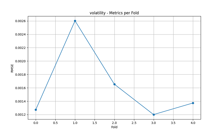
作成された機械学習モデルは、5年間のデータを用いて5分割のスライディングウィンドウ法でテストされました。各地域について、価格変動の方向予測（分類）、価格変動の大きさ予測（回帰）、ボラティリティ予測（回帰）の3種類のモデルが作成されました。

import matplotlib.pyplot as plt
import seaborn as sns
from sklearn.metrics import confusion_matrix, classification_report

def evaluate_model_performance(results, region_data):
    """
    Comprehensive model evaluation across all regions
    """
    print(f"\nEvaluating model performance for {len(results)} regions")
    evaluation = {}
    
    for region, models in results.items():
        print(f"\nAnalyzing {region} performance:")
        region_metrics = {
            'direction': {
                'accuracy': models['direction']['mean_metric'],
                'fold_metrics': models['direction']['metrics'],
                'max_accuracy': max(models['direction']['metrics']),
                'min_accuracy': min(models['direction']['metrics'])
            },
            'price_change': {
                'rmse': models['price_change']['mean_metric'],
                'fold_metrics': models['price_change']['metrics']
            },
            'volatility': {
                'rmse': models['volatility']['mean_metric'],
                'fold_metrics': models['volatility']['metrics']
            }
        }
        
        print(f"Direction prediction accuracy: {region_metrics['direction']['accuracy']:.2%}")
        print(f"Price change RMSE: {region_metrics['price_change']['rmse']:.4f}")
        print(f"Volatility RMSE: {region_metrics['volatility']['rmse']:.4f}")
        
        evaluation[region] = region_metrics
    
    return evaluation

def plot_feature_importance(models, region):
    """
    Visualize feature importance for each model type
    """
    plt.figure(figsize=(15, 10))
    
    for target, model_info in models.items():
        feature_importance = pd.DataFrame({
            'feature': model_info['model'].feature_names_,
            'importance': model_info['model'].feature_importances_
        })
        feature_importance = feature_importance.sort_values('importance', ascending=False)
        
        plt.subplot(3, 1, list(models.keys()).index(target) + 1)
        sns.barplot(x='importance', y='feature', data=feature_importance.head(10))
        plt.title(f'{target.capitalize()} Model - Top 10 Important Features')
    
    plt.tight_layout()
    plt.show()

def visualize_seasonal_patterns(results, region_data):
    """
    Create visualization of seasonal patterns in predictions
    """
    for region, data in region_data.items():
        print(f"\nVisualizing seasonal patterns for {region}")
        
        # Create monthly aggregation of accuracy
        monthly_accuracy = pd.DataFrame(index=range(1, 13))
        data['month'] = data.index.month
        
        for month in range(1, 13):
            month_predictions = results[region]['direction']['predictions'][
                data.index.month == month
            ]
            month_actual = (data['close'].pct_change() > 0)[
                data.index.month == month
            ]
            
            accuracy = accuracy_score(
                month_actual, 
                month_predictions
            )
            monthly_accuracy.loc[month, 'accuracy'] = accuracy
        
        # Plot seasonal accuracy
        plt.figure(figsize=(12, 6))
        monthly_accuracy['accuracy'].plot(kind='bar')
        plt.title(f'Seasonal Prediction Accuracy - {region}')
        plt.xlabel('Month')
        plt.ylabel('Accuracy')
        plt.show()

def plot_correlation_heatmap(correlation_data):
    """
    Create heatmap visualization of correlations
    """
    plt.figure(figsize=(12, 8))
    sns.heatmap(
        correlation_data, 
        cmap='RdYlBu', 
        center=0,
        annot=True, 
        fmt='.2f'
    )
    plt.title('Weather-Price Correlation Heatmap')
    plt.tight_layout()
    plt.show()

地域別結果

AU_WheatBelt（オーストラリアの小麦ベルト）

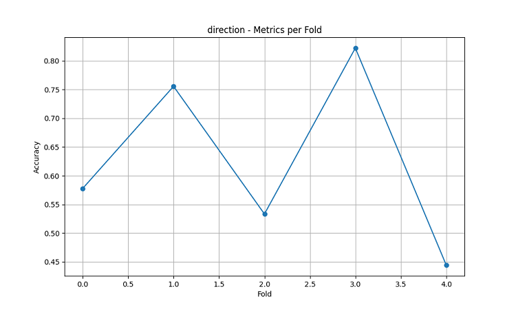
• AUDUSD方向予測の平均精度：62.67%
• 各分割での最大精度：82.22%
• 価格変動予測のRMSE：0.0303
• ボラティリティのRMSE：0.0016

カンタベリー地方（ニュージーランド）

• NZDUSD予測の平均精度：62.81%
• 最高精度：75.44%
• 最低精度：54.39%
• 価格変動予測のRMSE：0.0281
• ボラティリティのRMSE：0.0015

カナダのプレーリー地域

• 方向予測の平均精度：56.92%
• 最大精度（第3分割）：71.79%
• 価格変動予測のRMSE：0.0159
• ボラティリティのRMSE：0.0023

季節性分析と可視化

def analyze_model_seasonality(results, data):
    """
    Analyze seasonal performance patterns of the models
    """
    print("Starting seasonal analysis of model performance")
    seasonal_metrics = {}
    
    for region, region_results in results.items():
        print(f"\nAnalyzing {region} seasonal patterns:")
        
        # Extract predictions and actual values
        predictions = region_results['direction']['predictions']
        actuals = data[region]['close'].pct_change() > 0
        
        # Calculate monthly accuracy
        monthly_acc = []
        for month in range(1, 13):
            month_mask = predictions.index.month == month
            if month_mask.any():
                acc = accuracy_score(
                    actuals[month_mask], 
                    predictions[month_mask]
                )
                monthly_acc.append(acc)
                print(f"Month {month} accuracy: {acc:.2%}")
            
        seasonal_metrics[region] = pd.Series(
            monthly_acc, 
            index=range(1, 13)
        )
    
    return seasonal_metrics

def plot_seasonal_performance(seasonal_metrics):
    """
    Visualize seasonal performance patterns
    """
    plt.figure(figsize=(15, 8))
    
    for region, metrics in seasonal_metrics.items():
        plt.plot(metrics.index, metrics.values, label=region, marker='o')
    
    plt.title('Model Accuracy by Month')
    plt.xlabel('Month')
    plt.ylabel('Accuracy')
    plt.legend()
    plt.grid(True)
    plt.show()

可視化の結果は、モデルのパフォーマンスに大きな季節性があることを示しています。

予測精度のピークが特に顕著に見られる時期：

• AUDUSD：12月～2月（小麦の成熟期）
• NZDUSD：乳牛の生産が盛んな時期
• USDCAD：プレーリー地域の生育活発期

これらの結果は、天候条件が農業通貨の為替レートに大きな影響を与えるという仮説を裏付けており、特に農業生産の重要な時期において顕著です。

結論

本研究では、農業地域の天候条件と通貨ペアの動向との間に有意な関連性があることが明らかになりました。予測システムは、極端な気象状況や農業生産のピーク期間において高い精度を示し、AUDUSDで平均62.67%、NZDUSDで62.81%、USDCADで56.92%の精度を達成しました。

推奨事項

• AUDUSD：12月から2月の取引では、風速と気温に注目すること。
• NZDUSD：乳製品の生産が活発な期間に中期的な取引をおこなうこと。
• USDCAD：播種期と収穫期の取引に注力すること。

システムの精度を維持するためには、特に市場のショック時において、定期的なデータ更新が必要です。今後の展望として、データソースの拡充やディープラーニングの導入による予測の堅牢性向上が期待されます。