

Forecast Reconciliation (MinT): One Engine for Timeframe Hierarchies and Currency Graphs
 194
194
 0
0

Introduction
Open a chart with a multi-timeframe dashboard and you are looking at forecasts that contradict each other. The H1 model says one thing about the next few hours, the H4 model another about the same hours, and the D1 model a third about a window containing both. All three describe the same stretch of price, and rarely are any two consistent.
The usual answer is a weighted vote: give the higher timeframe more weight and tune until the dashboard agrees with your intuition. That produces one number, but says nothing about whether it beats the ones you started with.
The forecasting literature has an exact answer, and it is not a vote. It is called forecast reconciliation: when the targets are linearly related by construction, one way of making the forecasts consistent, the orthogonal projection, provably cannot increase total squared error. You do not need a better model, only to stop your models contradicting one another. The guarantee has conditions, which section 3 pins down and section 7 tests on real data.
We implement the method in pure MQL5, linear algebra included, and feed one engine two structures with nothing in common: a hierarchy of timeframes on one symbol, and a graph of currency pairs linked by the no-arbitrage identity. Then we measure what it does on years of real bars.
We will cover:
- The Contradiction in Your Own Forecasts
- Coherence as a Linear Constraint
- The Projection, and When It Cannot Hurt
- Choosing the Weight Matrix
- Building the Reconciliation Engine
- Two Hierarchies, One Summing Matrix
- Walk-Forward Evidence
- What the Reconciliation Residue Is Worth
- Watching It on a Chart
- Conclusion
The Contradiction in Your Own Forecasts
The script Recon_Inspect.mq5 builds a hierarchy, forecasts each node independently, and prints how far the forecasts sit from mutual consistency. Take EURUSD H1 and treat a day as twenty-four hourly returns. They sum into twelve two-hour returns, eight three-hour returns, and so on to one daily return: eight levels, sixty quantities, one stretch of price. Fit each level independently, as a trader running one model per chart does, and look at the sixty answers together.

Fig. 1. Timeframe models describing the same twenty-four hours, and the gap between them
On the run behind this article the sixty forecasts disagreed by 49.30 points RMS. The daily node forecast -213.78 points on its own evidence; consistent with the hourly stack, it would have been -370.47. That is a 156.69 point contradiction inside one dashboard, and nothing on the chart shows it.
The same happens across instruments, where the identity is arithmetic rather than a modelling choice. In log space currency pairs are additive: forecast EURUSD and USDJPY and you have implicitly forecast EURJPY. Recon_Inspect.mq5 prints, for twenty-one pairs, each quoted cross against the value its two USD legs imply, and they disagree.
The violations are a fraction of a pip, because one-step AR(1) forecasts of hourly returns sit near zero, and near-zero forecasts are nearly coherent. They are not zero, and each says that two of your models cannot both be right. The identity is exact for prices at one instant; on broker bars, where each close is that symbol's own last bid, it holds only approximately, and section 7 measures by how much.
Coherence as a Linear Constraint
Both situations have the same shape. There are n quantities to forecast, and they are not free: all are linear combinations of m underlying quantities. Write the targets as y and the underlying quantities as b:
y = S b
S is the summing matrix, n rows by m columns, recording only which combinations are forced. A vector satisfying this for some b is coherent, and the coherent vectors form an m-dimensional subspace of the n-dimensional space your forecasts live in.
For the temporal hierarchy the m free quantities are the twenty-four hourly returns of the coming day. The row for the two-hour block covering hours five and six holds ones in those columns; the daily row holds twenty-four. Eight factors give sixty rows over twenty-four columns.
   int row=0;
   for(int f=0; f<nf; f++)
     {
      const int k=factors[f];
      if(!AddLevelName(StringFormat("x%d",k)))
         return false;
      const int blocks=top_period/k;
      for(int j=0; j<blocks; j++)
        {
         for(int c=j*k; c<(j+1)*k; c++)
            m_S[(ulong)row][(ulong)c]=1.0;
         m_label[row] =StringFormat("x%d h%d",k,j+1);
         m_level[row] =f;
         m_factor[row]=k;
         m_step[row]  =j+1;
         row++;
        }
     }
   return true;
For the currency graph the free quantities are log prices against a numeraire. With USD as numeraire, every other currency gets one column, x_c = log(c/USD), and any pair is the difference of two columns:
log(EURJPY) = x_EUR - x_JPY = log(EURUSD) + log(USDJPY)
The right-hand form is the one a trader recognises, the middle one is what the matrix stores. Both hold on log returns as well as log prices, so one S serves both. Each row carries a +1 and a -1, or a single entry for a pair quoted against the numeraire.
   for(int s=0; s<ns; s++)
     {
      const string b=LegCurrency(symbols[s],true);
      const string q=LegCurrency(symbols[s],false);
      const int bi=CurrencyIndex(b);
      const int qi=CurrencyIndex(q);
      if(bi>=0)
         m_S[(ulong)s][(ulong)bi]= 1.0;
      if(qi>=0)
         m_S[(ulong)s][(ulong)qi]=-1.0;

      m_label[s] =symbols[s];
      m_level[s] =(b==numeraire || q==numeraire) ? 0 : 1;
      m_factor[s]=1;
      m_step[s]  =1;
     }
   return true;
The two constructions are unrelated, aggregation in time against arithmetic across instruments, yet both produce an n by m matrix of ones and minus ones that nothing downstream can tell apart.

Fig. 2. Timeframe aggregation and currency arithmetic assembling into the same object
The Projection, and When It Cannot Hurt
Now the claim. Given base forecasts yhat from any models, almost certainly incoherent, the reconciled forecast is
ytilde = S (S^T W^-1 S)^-1 S^T W^-1 yhat
where S^T is the transpose of S and W a weight matrix chosen in section 4. The result is coherent by construction, since it is S applied to something.
Why this helps is the argument the method rests on. The truth is coherent: realised hourly returns add up to the realised daily return, so the true vector lies in the subspace spanned by S, and your forecast vector generally does not. Every unit of forecast pointing out of the subspace is pure error. Strip that component off and nothing else, and what remains cannot be farther from the truth: that is the Pythagorean theorem, not a claim about markets. On the temporal hierarchy the premise is exact, since realised aggregates are sums of the same hourly returns; on the bar closes of the currency graph it is approximate, and section 7 prices the gap.

Fig. 3. The coherent subspace, an incoherent forecast, and the component that is guaranteed to be error
The formula does not look like a projection, but factorise W as L times its transpose, push S through the same factor, and it becomes ordinary least squares in whitened coordinates: the point in the column space of S closest to your forecast. Choosing W is choosing what "closest" means.
The geometric argument needs no statistics. The statistical result is due to Wickramasuriya, Athanasopoulos and Hyndman: with W equal to the covariance of the base forecast errors, the projection minimises the trace of the reconciled error covariance, a method called MinT, for minimum trace. That is a total over all n nodes, in expectation, not a promise about any one node or origin, a distinction section 8 measures. Its optimality is among unbiased reconciliations of unbiased base forecasts, and for the true covariance. You only ever have an estimate, and an AR(1) fitted on 120 observations is not exactly unbiased.
The geometric guarantee has its own conditions: a coherent truth, and error measured in the right geometry. For any positive definite W the projection is orthogonal in the metric W defines, so it cannot move you farther from a coherent truth by the W-weighted distance. Only for W equal to the identity is that ordinary squared error. Any other W tilts the projection relative to squared error; a good one buys accuracy, a bad one costs it, and section 7 shows the literature's W doing exactly that.
Three exact properties follow, and Recon_Inspect.mq5 measures them at the end of every run: a coherent input comes back unchanged, reconciling twice equals reconciling once, and the output satisfies the constraints:
projection invariants, largest difference relative to the widest node
  coherent input returned unchanged : 5.803e-16
  reconciling twice equals once     : 2.176e-16
  output satisfies the constraints  : 1.777e-15
Those are single units in the last place of a double, which is what exact looks like in floating point. The third check uses an independent projector, so it cannot flatter itself; anything materially larger is a bug.
Choosing the Weight Matrix
Coherence and those invariants hold for any positive definite W. What W decides is whether the projection is any good, and this is where an implementation works or quietly destroys its input. The library offers five options, ordered by how much they claim to know about the errors.
| Scheme | W | What it assumes |
|---|---|---|
| OLS | Identity | Nothing. Every node's error is equally important and independent. |
| WLS-struct | diag(S times 1) | A node aggregating twelve hours has more variance than one aggregating one. Needs no data. |
| WLS-var | diag of sample covariance | Per-node error variances, measured, but no correlations. |
| MinT-sample | Sample covariance | The full error covariance, taken at face value. |
| MinT-shrink | Shrunk covariance | The full covariance, with the correlations regularised. |
One function assembles all five: two need only the shape of S, and the other three delegate to the covariance estimator.
//+------------------------------------------------------------------+
//| Assemble the weight matrix for one scheme.                       |
//|                                                                  |
//|  The structural weights deserve a note. They set each node's     |
//|  weight to the number of bottom quantities it aggregates, which  |
//|  needs no data at all and encodes the one thing that is true by  |
//|  construction: a node summing twelve hours of return has more    |
//|  variance to be wrong about than a node summing one. It is the   |
//|  scheme to fall back on while the error store is still filling.  |
//+------------------------------------------------------------------+
bool CReconciler::BuildWeight(const ENUM_REC_WEIGHT scheme,
                              CCovarianceEstimator &est,matrix &W)
  {
   const ulong n=(ulong)m_n;
   m_lambda=0.0;

   if(scheme==REC_W_OLS)
     {
      W=matrix::Zeros(n,n);
      for(ulong i=0; i<n; i++)
         W[i][i]=1.0;
      return true;
     }

   if(scheme==REC_W_WLS_STRUCT)
     {
      W=matrix::Zeros(n,n);
      for(ulong i=0; i<n; i++)
        {
         double rowsum=0.0;
         for(ulong j=0; j<(ulong)m_m; j++)
            rowsum+=MathAbs(m_S[i][j]);
         W[i][i]=(rowsum>0.0 ? rowsum : 1.0);
        }
      return true;
     }

   if(est.Dim()!=m_n)
     {
      PrintFormat("CReconciler: error store holds %d nodes, hierarchy has %d",
                  est.Dim(),m_n);
      return false;
     }

   switch(scheme)
     {
      case REC_W_WLS_VAR:
         return est.Diagonal(W);
      case REC_W_MINT_SAMPLE:
         return est.Sample(W);
      case REC_W_MINT_SHRINK:
         return est.Shrink(W,m_lambda);
     }
   return false;
  }
The two data-free schemes return before the estimator is consulted, so a caller can reconcile from the first origin instead of waiting for an error store to fill; otherwise an indicator would plot nothing for its first eighty blocks.
The other three need the covariance of past base forecast errors, and that estimate is fragile. Sixty nodes mean 1,830 free parameters, and one residual vector per day needs sixty trading days, about three months, just to reach full rank. The projection inverts it, so an immature estimate amplifies exactly the directions that are pure noise:
//+------------------------------------------------------------------+
//| Unbiased sample covariance over the stored window.               |
//+------------------------------------------------------------------+
bool CCovarianceEstimator::Sample(matrix &cov) const
  {
   vector mean, sd;
   if(!Moments(mean,sd))
      return false;

   cov=matrix::Zeros((ulong)m_dim,(ulong)m_dim);
   for(int t=0; t<m_count; t++)
     {
      const int s=Slot(t);
      for(int i=0; i<m_dim; i++)
        {
         const double di=m_obs[(ulong)s][(ulong)i]-mean[(ulong)i];
         for(int j=i; j<m_dim; j++)
           {
            const double dj=m_obs[(ulong)s][(ulong)j]-mean[(ulong)j];
            cov[(ulong)i][(ulong)j]+=di*dj;
           }
        }
     }
   const double denom=(double)(m_count-1);
   for(int i=0; i<m_dim; i++)
     {
      for(int j=i; j<m_dim; j++)
        {
         const double v=cov[(ulong)i][(ulong)j]/denom;
         cov[(ulong)i][(ulong)j]=v;
         cov[(ulong)j][(ulong)i]=v;
        }
     }
   return true;
  }
Nothing there can fail or warn: it returns a well-formed matrix whose smallest eigenvalues are noise. The standard fix, and the one the MinT paper uses, is Schaefer and Strimmer's estimator, which shrinks the off-diagonal correlations toward zero by an analytically chosen intensity:
lambda = sum var(r_ij) / sum r_ij^2, over i != j
The numerator measures how uncertain the sample correlations are and the denominator how large, so pure noise is shrunk away and precise correlations survive. The diagonal is never touched: it carries the scale difference between hourly and daily nodes, and shrinking it would flatten the hierarchy.
//--- variance of each off-diagonal correlation across the window.
   double num=0.0, den=0.0;
   for(ulong i=0; i<n; i++)
     {
      for(ulong j=i+1; j<n; j++)
        {
         const double wbar=r[i][j]*(T-1.0)/T;
         double acc=0.0;
         for(int t=0; t<m_count; t++)
           {
            const double w=z[(ulong)t][i]*z[(ulong)t][j];
            acc+=(w-wbar)*(w-wbar);
           }
         num+=T/((T-1.0)*(T-1.0)*(T-1.0))*acc;
         den+=r[i][j]*r[i][j];
        }
     }

   lambda=(den>0.0 ? num/den : 1.0);
   lambda=MathMax(0.0,MathMin(1.0,lambda));

Fig. 4. Correlation shrinkage as the intensity rises from zero to one
Building the Reconciliation Engine
The engine, Reconcile.mqh, knows nothing about markets: it receives a summing matrix and a weighting and does arithmetic, which is why one object serves both hierarchies unchanged.
The numerical care goes into never forming W inverse. A covariance estimated from a few hundred observations at sixty dimensions is routinely near-singular, and a general inverse returns numbers rather than an error. Every solve therefore goes through a Cholesky factorisation, which fails loudly on a matrix that is not positive definite, with a ridge escalating by powers of ten until it succeeds. The ridge is reported because it changes the problem: with ridge r the projection is the one for W + rI. At the seed size that is hygiene; when large, it is a different weighting and the sign of a nearly rank-deficient covariance.
   double ridge=0.0;
   for(int attempt=0; attempt<REC_RIDGE_TRIES; attempt++)
     {
      L=matrix::Zeros(n,n);
      bool ok=true;
      for(ulong i=0; i<n && ok; i++)
        {
         for(ulong j=0; j<=i; j++)
           {
            double s=A[i][j];
            if(i==j)
               s+=ridge;
            for(ulong k=0; k<j; k++)
               s-=L[i][k]*L[j][k];
            if(i==j)
              {
               if(s<=0.0 || !MathIsValidNumber(s))
                 {
                  ok=false;
                  break;
                 }
               L[i][i]=MathSqrt(s);
              }
            else
               L[i][j]=s/L[j][j];
           }
        }
      if(ok)
        {
         ridge_used=ridge;
         return true;
        }
      ridge=(ridge==0.0 ? REC_RIDGE_SEED*scale : ridge*10.0);
     }
   return false;
Only one place forms an inverse explicitly, and its header says where it may be used:
//+------------------------------------------------------------------+
//| Inverse of a symmetric positive definite matrix, by solving      |
//| against each unit vector in turn. Only ever called on the small  |
//| m x m normal-equation matrix, never on W itself. It inherits the |
//| conditioning of W, so any ridge it needed is handed back too.    |
//+------------------------------------------------------------------+
bool RecSpdInverse(const matrix &A,matrix &Ainv,double &ridge_used)
  {
   matrix L;
   if(!RecCholeskyRidge(A,L,ridge_used))
      return false;
   const ulong n=A.Rows();
   Ainv=matrix::Zeros(n,n);
   for(ulong j=0; j<n; j++)
     {
      vector e=vector::Zeros(n), t, col;
      e[j]=1.0;
      if(!RecSolveLowerVec(L,e,t) || !RecSolveUpperVec(L,t,col))
         return false;
      for(ulong i=0; i<n; i++)
         Ainv[i][j]=col[i];
     }
   return true;
  }
The matrix inverted is the m by m normal-equation matrix, twenty-four rows for the temporal hierarchy and seven for the currency one, not an estimated covariance. That is far less fragile: it is small, the connectivity check of section 6 guarantees its rank, and any ridge it needs, since it inherits the conditioning of W, is reported too. Preparation whitens S, inverts that small matrix and caches one m by n mapping G, so each reconciliation then costs two matrix-vector products:
//+------------------------------------------------------------------+
//| Factorise W and cache everything the per-bar path needs.         |
//|                                                                  |
//|  W is never inverted. It is factorised as L Lt, S is pushed      |
//|  through the same factor to give Stilde, and the reconciliation  |
//|  then reduces to an ordinary least squares problem in the        |
//|  whitened coordinates. That is not only more stable than forming |
//|  W^-1, it is the reason the result is recognisably a projection  |
//|  rather than a formula: in whitened space MinT is exactly the    |
//|  orthogonal projection onto the column space of S.               |
//+------------------------------------------------------------------+
bool CReconciler::Factorise(const matrix &W)
  {
   const ulong n=(ulong)m_n, m=(ulong)m_m;

   matrix L;
   if(!RecCholeskyRidge(W,L,m_ridge))
     {
      Print("CReconciler: weight matrix is not positive definite");
      return false;
     }
   m_L=L;

//--- Stilde = L^-1 S, the summing matrix in whitened coordinates.
   matrix Stilde;
   if(!RecSolveLower(L,m_S,Stilde))
      return false;

//--- A = Stilde^T Stilde = S^T W^-1 S, the normal-equation matrix.
   matrix StildeT, A;
   RecTranspose(Stilde,StildeT);
   if(!RecMatMul(StildeT,Stilde,A))
      return false;
   if(!RecSpdInverse(A,m_Ainv,m_ridge_a))
     {
      Print("CReconciler: summing matrix is rank deficient");
      return false;
     }

//--- M = Stilde^T L^-1 = S^T W^-1, obtained column by column so that
//--- no explicit inverse of L is ever formed.
   matrix Mt=matrix::Zeros(n,m);
   for(ulong j=0; j<m; j++)
     {
      vector col=vector::Zeros(n), sol;
      for(ulong i=0; i<n; i++)
         col[i]=Stilde[i][j];
      if(!RecSolveUpperVec(L,col,sol))
         return false;
      for(ulong i=0; i<n; i++)
         Mt[i][j]=sol[i];
     }
   matrix Mm;
   RecTranspose(Mt,Mm);

   if(!RecMatMul(m_Ainv,Mm,m_G))
      return false;

   m_ready=true;
   return true;
  }
Everything expensive is now done. The per-bar path is two short functions, the first recovering the bottom level:
//+------------------------------------------------------------------+
//| The m free quantities implied by a set of base forecasts.        |
//+------------------------------------------------------------------+
bool CReconciler::BottomLevel(const vector &yhat,vector &bhat) const
  {
   if(!m_ready || (int)yhat.Size()!=m_n)
      return false;
   return RecMatVec(m_G,yhat,bhat);
  }
The second sums it back up through S, which is the projection itself:
//+------------------------------------------------------------------+
//| Project onto the coherent subspace: reconstruct the bottom level |
//| that best explains the base forecasts, then sum it back up.      |
//+------------------------------------------------------------------+
bool CReconciler::Reconcile(const vector &yhat,vector &ytilde) const
  {
   vector bhat;
   if(!BottomLevel(yhat,bhat))
      return false;
   return RecMatVec(m_S,bhat,ytilde);
  }
The cached mapping also gives the covariance of the reconciled errors, the basis of coherent forecast intervals. With a coherent truth the reconciled error is P = S G times the base error, so base errors of covariance Sigma become P Sigma P^T. The familiar shortcut S (S^T W^-1 S)^-1 S^T equals that only when W is Sigma, which for OLS and the structural weights it never is, so the function takes Sigma from the caller:
//+------------------------------------------------------------------+
//| Covariance of the reconciled errors, P Sigma P^T with P = S G,   |
//| for base errors of covariance Sigma. It equals S A^-1 S^T only   |
//| when W is Sigma itself, so Sigma is passed in, not assumed.      |
//+------------------------------------------------------------------+
bool CReconciler::ReconciledCovariance(const matrix &base_cov,matrix &cov) const
  {
   if(!m_ready || base_cov.Rows()!=(ulong)m_n || base_cov.Cols()!=(ulong)m_n)
      return false;
   matrix P, PT, tmp;
   if(!RecMatMul(m_S,m_G,P))
      return false;
   RecTranspose(P,PT);
   if(!RecMatMul(P,base_cov,tmp))
      return false;
   return RecMatMul(tmp,PT,cov);
  }
Two Hierarchies, One Summing Matrix
Hierarchy.mqh is the only file that knows what the constraints mean. Beyond the two builders of section 2, it handles three ways a summing matrix can be well formed and still describe something untrue.
The currency graph can be rank deficient. If a currency is unreachable from the numeraire, S loses rank and the escalating ridge quietly invents an answer. A union-find pass catches this before any data is loaded and names the stranded currency; the parent array is one slot longer than the currency list so the numeraire has somewhere to sit:
//--- slot m is the numeraire, which is why the array is one longer.
   int parent[];
   ArrayResize(parent,m+1);
   for(int i=0; i<=m; i++)
      parent[i]=i;

   for(int s=0; s<ArraySize(symbols); s++)
     {
      const string b=LegCurrency(symbols[s],true);
      const string q=LegCurrency(symbols[s],false);
      int a=(b==numeraire ? m : CurrencyIndex(b));
      int c=(q==numeraire ? m : CurrencyIndex(q));
      if(a<0 || c<0)
         continue;
      while(parent[a]!=a)
         a=parent[a];
      while(parent[c]!=c)
         c=parent[c];
      if(a!=c)
         parent[a]=c;
     }

   int root=m;
   while(parent[root]!=root)
      root=parent[root];
   for(int i=0; i<m; i++)
     {
      int r=i;
      while(parent[r]!=r)
         r=parent[r];
      if(r!=root)
        {
         PrintFormat("CHierarchy: %s is not reachable from %s",
                     m_bottom[i],numeraire);
         return false;
        }
     }
   return true;
It costs microseconds once per session, and buys the difference between a run that fails and a run that lies.
Bars are not aligned across symbols. A naive CopyRates per symbol plus index arithmetic silently compares a EURJPY bar with a EURUSD bar from a different hour whenever one had no ticks. The loader keys on bar open time, keeps only times present in every symbol and reports the rest: two bars of twelve thousand in section 7, but 3,504 in an earlier session before the terminal had back-filled every pair. The first symbol's times are the candidate timeline, and every other symbol confirms or strikes each one:
   for(int s=1; s<ns; s++)
     {
      const int gs=CopyRates(symbols[s],tf,1,bars,rates);
      if(gs<8)
        {
         PrintFormat("CAlignedBars: %s returned %d bars",symbols[s],gs);
         return false;
        }
      int p=0;
      for(int i=0; i<got; i++)
        {
         while(p<gs && rates[p].time<cand[i])
            p++;
         if(p<gs && rates[p].time==cand[i])
            raw[(ulong)i][(ulong)s]=rates[p].close;
         else
            keep[i]=false;
        }
     }
A missing time does not shift the rows up; it marks that instant unusable for every symbol at once. Alignment makes bars comparable, not the identity exact: each close is that symbol's last bid in the hour, last ticks arrive at different moments and spreads differ, so the realised cross and its legs still disagree slightly. Section 7 measures by how much.
The library never sleeps. It loads whatever history the terminal has, and a caller needing more must wait itself. An indicator runs on the interface thread, where a wait loop copied from a script never yields and the plot silently never appears.
Since every claim rests on S being the matrix you think it is, it is worth printing. Its entries are only 0, 1 or -1, so one character per column fits even sixty rows on a log line:
//+------------------------------------------------------------------+
//| Print S compactly. Entries are only ever 0, 1 or -1, so one      |
//| character per column keeps even a sixty-row matrix readable.     |
//+------------------------------------------------------------------+
void PrintSummingMatrix(CHierarchy &h)
  {
   matrix S;
   h.GetSummingMatrix(S);
   string head="                 ";
   for(int j=0; j<h.M(); j++)
      head+=StringSubstr(h.BottomName(j)+"   ",0,1);
   PrintFormat("%s   (columns: %s ...)",head,h.BottomName(0));
   for(int i=0; i<h.N(); i++)
     {
      string row="";
      for(int j=0; j<h.M(); j++)
        {
         const double v=S[(ulong)i][(ulong)j];
         row+=(v>0.5 ? "+" : (v<-0.5 ? "-" : "."));
        }
      PrintFormat("%-16s %s",h.Label(i),row);
     }
  }
Walk-Forward Evidence
The theorem needs no empirical confirmation, but it makes checkable predictions and is silent on what a user wants to know: how much the projection helps, and what the other weightings do. Recon_Evidence.mq5 measures both, origin by origin. It walks forward one top period at a time: each level is refitted on its own past and forecast across the coming period, realised aggregates are formed once it has happened, and the residual enters the error store only after scoring. That ordering is the no-lookahead argument:
         //--- every column is scored on the same origin or none of them is,
         //--- otherwise the loss differentials would not be paired.
         if(rec[4].IsReady())
           {
            matrix pred=matrix::Zeros(REC_NCOL,(ulong)n);
            for(int i=0; i<n; i++)
               pred[0][(ulong)i]=yhat[(ulong)i];
            bool good=true;
            for(int s=0; s<5 && good; s++)
              {
               vector yt;
               good=rec[s].Reconcile(yhat,yt);
               if(good)
                  for(int i=0; i<n; i++)
                     pred[(ulong)(s+1)][(ulong)i]=yt[(ulong)i];
              }
            if(good)
              {
               ev.Origin(y,pred,level,n);
               ev.NoteGuarantee(rec,y,pred,n);
               vector bs=vector::Zeros((ulong)n), rc=vector::Zeros((ulong)n);
               for(int i=0; i<n; i++)
                 {
                  bs[(ulong)i]=pred[0][(ulong)i];
                  rc[(ulong)i]=pred[(ulong)bcol][(ulong)i];
                 }
               st.Add(y,bs,rc,n);
              }
           }
        }

      //--- the residual enters the store only now that it has been
      //--- scored, which is what keeps the weights strictly historical.
      vector e=vector::Zeros((ulong)n);
      for(int i=0; i<n; i++)
         e[(ulong)i]=y[(ulong)i]-yhat[(ulong)i];
      est.Push(e);
All five schemes are scored on an origin or none is, because the Diebold-Mariano test compares paired losses, and a column that skipped its hard origins would win. And est.Push comes last: move it three lines earlier and every number becomes a lookahead.
A top period here is twenty-four consecutive H1 bars counted back from the latest close, not a calendar day, so a block can span a weekend. Twenty-four consecutive returns still sum to their total, so the identity holds, but "daily node" means the twenty-four-bar node. The indicator of section 9 aligns its blocks to the server's day.
The base forecasters are deliberately plain: a last-value forecast that repeats the most recent return, a window mean, and a fitted AR(1). A strong model would let any gain be credited to the model rather than to reconciliation:
//+------------------------------------------------------------------+
//| Forecast h steps ahead from the end of the supplied history.     |
//|                                                                  |
//|  The AR(1) coefficient is clipped short of the unit circle. An   |
//|  unclipped estimate near one turns the h-step forecast into an   |
//|  extrapolation that grows with the horizon, and on the coarser   |
//|  aggregation levels, where a fit sees only a few dozen           |
//|  observations, that happens often enough to dominate the error   |
//|  of the whole hierarchy.                                         |
//+------------------------------------------------------------------+
double CBaseForecaster::Forecast(const double &x[],const int count,const int h) const
  {
   if(count<4 || h<1 || count>ArraySize(x))
      return 0.0;
   const int w=MathMin(m_window,count);
   if(w<4)
      return 0.0;

   if(m_model==REC_BASE_NAIVE)
      return x[count-1];

   const double mu=WindowMean(x,count,w);
   if(m_model==REC_BASE_DRIFT)
      return mu;

   double num=0.0, den=0.0;
   for(int i=count-w+1; i<count; i++)
     {
      const double a=x[i-1]-mu;
      num+=a*(x[i]-mu);
      den+=a*a;
     }
   if(den<=0.0)
      return mu;

   double phi=num/den;
   phi=MathMax(-0.95,MathMin(0.95,phi));
   return mu+MathPow(phi,h)*(x[count-1]-mu);
  }
The clip on phi is the one line that is not textbook, and its header says why. Replace this function with your own model and nothing else needs to change.
All runs use bid closes from a server whose clock follows the New York close (GMT+3 at the time). Here is EURUSD H1 over the 60,000 bars from February 2017 to October 2026: 2,087 scored origins, AR(1) base forecasts, and weights refitted every origin from a rolling window of 750 residuals. Rows run from the hourly nodes (x1) to the daily node (x24), with ALL pooling every node; the scheme columns give the change in mean squared error, so negative is better.
| Level | Base RMSE, bp | OLS | WLS-struct | WLS-var | MinT-sample | MinT-shrink |
|---|---|---|---|---|---|---|
| x1 | 9.443 | -0.75% | -0.68% | -0.69% | +93.64% | -0.60% |
| x2 | 13.135 | -0.89% | -0.75% | -0.76% | +88.44% | -0.77% |
| x3 | 16.030 | -0.65% | -0.39% | -0.41% | +94.08% | -0.58% |
| x4 | 18.401 | -0.52% | -0.21% | -0.22% | +110.45% | -0.52% |
| x6 | 22.578 | -0.20% | +0.26% | +0.22% | +83.62% | -0.18% |
| x8 | 25.969 | -0.47% | +0.16% | +0.14% | +153.08% | -0.61% |
| x12 | 31.539 | -0.77% | +0.16% | +0.11% | +105.73% | -0.90% |
| x24 | 43.925 | +0.11% | +2.25% | +2.17% | +144.52% | +0.23% |
| ALL | 16.472 | -0.52% | +0.08% | +0.05% | +108.77% | -0.50% |
| Diebold-Mariano | - | 25.82 | -0.55 | -0.37 | -1.33 | 4.11 |
Five things stand out.
- The improvement is not noise. OLS cuts pooled mean squared error by 0.52%, with a Diebold-Mariano statistic of 25.82 and p below 0.0001 over 2,087 origins.
- The gain is uneven. OLS gains most on the finest levels, -0.75% and -0.89% at x1 and x2, between -0.20% and -0.77% in the middle, and turns into a small loss, +0.11%, at the daily node. Section 8 magnifies that last cell.
- Textbook MinT is dangerous here. The sample-covariance version inflated error by 108.77%; on a 250-residual window over the latest 30,000 bars by 830%, and on that window ending six weeks earlier by over 3,700%. The damage is as unstable as the estimate, which needed a ridge in 1,851 of 2,087 refits despite 750 residuals for sixty nodes: numerically singular most of the time, as section 4 predicted. Shrinkage repairs the long window, -0.50% at p below 0.0001 with intensity averaging 0.056, but on the short one reaches only -0.13% (p = 0.23) at intensity 0.149.
- The two WLS columns are one column. They never differ by as much as a tenth of a percent: the measured variances are proportional to the structural row sums, so the free estimate already knows what the measured one learns.
- OLS was the safe choice here. It has no covariance to get wrong and never blew up; MinT-shrink matched it, -0.50% against -0.52%, and beat it at x8 and x12. With the naive forecasts of section 8 both MinT variants beat OLS outright, -32.9% and -33.3% against -24.8%. Two hierarchies and three simple models cannot crown a general default; what survives both runs is that MinT buys its advantage with an estimate, and OLS cannot be charged for a bad one.
Every p-value comes from one function:
//+------------------------------------------------------------------+
//| Diebold-Mariano test on a loss differential.                     |
//|                                                                  |
//|  d[t] is loss(base) - loss(reconciled), so a positive mean is    |
//|  reconciliation winning. The long-run variance uses a Bartlett   |
//|  kernel out to 'lag', the Harvey, Leybourne and Newbold factor   |
//|  corrects its small-sample bias, and the p-value is read from    |
//|  Student's t with n-1 degrees of freedom, as they recommend.     |
//+------------------------------------------------------------------+
bool RecDieboldMariano(const double &d[],const int n,const int lag,
                       double &stat,double &pval)
  {
   stat=0.0;
   pval=1.0;
   if(n<8)
      return false;

   double mean=0.0;
   for(int i=0; i<n; i++)
      mean+=d[i];
   mean/=n;

   const int L=(int)MathMax(0,MathMin(lag,n-2));
   double gamma0=0.0;
   for(int i=0; i<n; i++)
      gamma0+=(d[i]-mean)*(d[i]-mean);
   gamma0/=n;

   double lrv=gamma0;
   for(int k=1; k<=L; k++)
     {
      double g=0.0;
      for(int i=k; i<n; i++)
         g+=(d[i]-mean)*(d[i-k]-mean);
      g/=n;
      lrv+=2.0*(1.0-(double)k/(double)(L+1))*g;
     }
   if(lrv<=0.0 || !MathIsValidNumber(lrv))
      return false;

   const double h=(double)(L+1);
   const double raw=mean/MathSqrt(lrv/(double)n);
   const double corr=MathSqrt((n+1.0-2.0*h+h*(h-1.0)/n)/(double)n);
   stat=raw*corr;
   int err=0;
   pval=2.0*MathCumulativeDistributionT(MathAbs(stat),n-1.0,false,false,err);
   return (err==0 && MathIsValidNumber(pval));
  }
The Bartlett long-run variance and the small-sample factor both make the test more conservative, and the p-value comes from Student's t with n-1 degrees of freedom, as Harvey, Leybourne and Newbold recommend. The loss differential is one number per origin, the mean squared error across nodes, so same-date dependence between nodes is absorbed before the test. Nor do the hourly nodes dominate it: each level contributes 11.9% to 13.1% of pooled error, since per-node variance grows with width about as fast as the node count shrinks.
The currency hierarchy tells a consistent story. It covers the seven USD majors and fourteen crosses (EURJPY, EURGBP, EURCHF, EURAUD, GBPJPY, AUDJPY, CADJPY, CHFJPY, AUDNZD, AUDCAD, GBPCAD, GBPCHF, EURCAD, NZDJPY) over 12,000 H1 bars from October 2024 to October 2026, with AR(1) forecasts one bar ahead and a 1,500-residual window refitted every 24 bars. Over 11,077 origins OLS cuts pooled error by 0.48% at a statistic of 12.78, and the crosses gain more than the legs, -0.53% against -0.40%, since a cross carries two constrained legs. MinT-sample costs 1.09% here rather than 109%. That contrast suggests a dimensionality problem, but the runs also differ in data, errors, window and how coherent the truth is, so it is not proof; what the temporal run shows on its own is a covariance estimate that was numerically singular most of the time.
Checking the theorem origin by origin
A pooled percentage averages over origins; the geometric guarantee is about each one. NoteGuarantee, called right after scoring, asks every scheme at every origin whether reconciling moved the forecast farther from the outcome, in squared error and in its own W-weighted distance. It also projects the realised outcome, to measure how far the truth sits from coherent:
//+------------------------------------------------------------------+
//| Check the guarantee at one origin. Each scheme may not move      |
//| farther from a coherent truth in its own metric; the OLS         |
//| residue of the truth says how coherent the truth really was.     |
//+------------------------------------------------------------------+
void CEvidence::NoteGuarantee(CReconciler &rec[],const vector &y,
                              const matrix &pred,const int n)
  {
   vector eb=vector::Zeros((ulong)n), er=vector::Zeros((ulong)n);
   for(int s=0; s<REC_NCOL-1; s++)
     {
      for(int i=0; i<n; i++)
        {
         eb[(ulong)i]=y[(ulong)i]-pred[0][(ulong)i];
         er[(ulong)i]=y[(ulong)i]-pred[(ulong)(s+1)][(ulong)i];
        }
      double db=0.0, dr=0.0;
      if(rec[s].WeightedDistance(eb,db) && rec[s].WeightedDistance(er,dr)
         && dr>db*(1.0+1.0e-9))
         m_rise_w[s+1]++;
      if(rec[s].Scheme()==REC_W_OLS)
        {
         const double r=rec[s].Incoherence(y);
         m_truth_sq+=r*r;
        }
     }
  }
Origins at which each scheme moved farther from the outcome:
| Scheme | Temporal, squared error (of 2,087) | Temporal, own metric (of 2,087) | Currency, squared error (of 11,077) | Currency, own metric (of 11,077) |
|---|---|---|---|---|
| OLS | 0 | 0 | 609 | 609 |
| WLS-struct | 970 | 0 | 3,793 | 604 |
| WLS-var | 972 | 0 | 3,946 | 654 |
| MinT-sample | 1,227 | 0 | 5,817 | 474 |
| MinT-shrink | 936 | 0 | 4,993 | 527 |
- On the temporal hierarchy the theorem holds at every origin. OLS was worse on none of 2,087 days, and none of 2,407 with the naive forecasts of section 8, as predicted for a truth measured 0.0000 bp from the coherent subspace.
- Every weighting keeps its own promise; only OLS promises anything about squared error. All five schemes moved closer to the truth in their own metric at every temporal origin. MinT-sample still worsened squared error at 1,227 of them, by 109% in total: it did what the maths promises, in a geometry no trader cares about.
- On the currency graph the truth is not coherent. Realised bar returns sit 0.60 bp RMS off the coherent subspace, 0.37% of the base mean squared error. OLS was worse at 609 of 11,077 hours, 5.5%, yet cut pooled error by 0.48%.
Write the realised vector as y = y_c + y_perp, a coherent part plus a residue, and let P be the orthogonal projector. Reconciliation can then lose at most the residue:
|P yhat - y|^2 <= |yhat - y|^2 + |y_perp|^2
On the temporal hierarchy y_perp is zero and the bound is the theorem. On the currency graph it answers how exact the no-arbitrage identity is on broker bars: about 0.6 bp per hour, small beside a 10 bp forecast error, but of the same order as the gain.
What the Reconciliation Residue Is Worth
Reconciliation produces one number per origin that it has no use for: the size of the correction, or how far the base forecasts sat from coherence. The literature discards it. Does it predict anything?
CIncoherenceStudy sorts origins by that residue into equal buckets and scores base against reconciled inside each, in squared error and in directional hit rate, since the two can disagree. If the residue is inert, the relationship is the same in every bucket.
      const double yi=y[(ulong)i];
      const double bi=base[(ulong)i];
      const double ri=rec[(ulong)i];
      const double d =bi-ri;
      gap+=d*d;
      sb +=(yi-bi)*(yi-bi);
      sr +=(yi-ri)*(yi-ri);

      //--- a realised move of exactly zero has no sign to agree with.
      if(yi==0.0)
         continue;
      sg+=1.0;
      if((yi>0.0)==(bi>0.0))
         hb+=1.0;
      if((yi>0.0)==(ri>0.0))
         hr+=1.0;
The run below uses the same hierarchy and bars with naive base forecasts and OLS. Naive forecasts are far more incoherent, so the effect is plain: a pooled improvement of 24.8% against the 0.52% of section 7, the same mechanism at another amplitude. Over 2,407 origins the gradient is clean and monotone.
| Bucket | Origins | Incoherence, bp | Base RMSE | Reconciled RMSE | MSE change | Base hit | Reconciled hit |
|---|---|---|---|---|---|---|---|
| 1 (calmest) | 481 | 3.289 | 14.863 | 14.473 | -5.17% | 49.12% | 49.43% |
| 2 | 481 | 5.258 | 17.358 | 16.532 | -9.29% | 49.92% | 50.14% |
| 3 | 482 | 6.983 | 17.864 | 16.431 | -15.41% | 49.76% | 50.28% |
| 4 | 481 | 9.636 | 21.538 | 19.225 | -20.33% | 49.63% | 48.64% |
| 5 (noisiest) | 482 | 19.083 | 36.957 | 29.759 | -35.16% | 49.50% | 48.58% |
The residue tracks the gain. Reconciliation removes almost seven times more squared error in the noisiest bucket than in the calmest, monotonically across all five. That is the central lesson as a measurement: reconciliation removes error in proportion to the contradiction you were carrying.
The gradient is not a signal, though. The bucket edges are whole-sample quantiles:
   double sorted[];
   ArrayResize(sorted,m_count);
   ArrayCopy(sorted,m_incoh,0,0,m_count);
   ArraySort(sorted);

   double edge[];
   ArrayResize(edge,nb-1);
   for(int k=0; k<nb-1; k++)
      edge[k]=sorted[(int)((double)(k+1)*m_count/nb)-1];
Classifying one origin therefore requires origins that had not yet happened. This is an ex post association, not a validated predictor: it establishes what the residue is, the contradiction reconciliation had available to remove. Since the residue is known at the origin, expanding-window edges could test it as a predictor; that test is not run here.
It also says something less comfortable. Here is the same run scored on the daily node alone:
| Bucket | MSE change |
|---|---|
| 1 (calmest) | -1.59% |
| 2 | +1.37% |
| 3 | +5.49% |
| 4 | +14.40% |
| 5 (noisiest) | +79.43% |
The sign flips. Where the pooled column fell to -35.16%, this one crosses over by the second bucket and climbs with the residue: in the top bucket the total improves by 35% while the daily node gets 79% worse. Section 3 warned of this. The projection minimises a trace, a sum free to buy a large reduction in fifty-nine terms with an increase in the sixtieth, and the widest node, aggregating all twenty-four bottom quantities, is the cheapest place to put the error.
The currency hierarchy confirms the mechanism by its absence: no node aggregates more than two free quantities, so there is nowhere cheap to hide error, and NZDJPY's squared error moves by at most three hundredths of a percent in any bucket.

Fig. 5. The trace tradeoff: error removed from fifty-nine nodes and pushed into one
Two more observations. First, incoherence belongs to your forecasting procedure, not to the market. A naive forecast on the currency graph repeats the last returns, which satisfy the identity up to the bar-close residue, so it is nearly coherent; on the temporal hierarchy each level's last observation spans a different window, so it is wildly incoherent. Same model, market and engine: mean incoherence of 0.30 bp against 8.85, and gains of -0.29% against -24.8%.
Second, the reason for the scope note: pooled hit rates sit between 48.6% and 50.3%, flat across buckets and unmoved by reconciliation, and on the daily node they scatter from 47.3% to 52.8% with no ordering, which is sampling noise on a few hundred coin flips. These simple models carry no measurable directional information on this sample, before or after reconciliation. The method improves how close you are on average, not how often you are on the right side.
Watching It on a Chart
ReconciledForecast.mq5 plots, in a separate window, the base forecast (buffer 0, dotted silver), the reconciled forecast (buffer 1, solid blue) and the incoherence (buffer 2, red histogram) for one node of the temporal hierarchy, all in points so they read against the chart.
Inputs
| Input | Default | What it does |
|---|---|---|
| InpTopPeriod | 24 | Chart bars in one top period. On H1 the default makes the top node a full day |
| InpFactors | 1,2,3,4,6,8,12,24 | Aggregation levels. Every factor must divide InpTopPeriod exactly, and at least two are required |
| InpShowFactor | 24 | Aggregation level of the node to plot. 24 is the daily node, 1 an individual hour |
| InpShowStep | 1 | Which block within that level. With factor 4 the values 1 to 6 select the six four-hour blocks of the day |
| InpShowIncoh | true | Draw the incoherence histogram. Turning it off leaves the two forecast lines on their own scale |
| InpModel | AR(1) | Base model fitted per node: last value, window mean or AR(1) |
| InpFitWindow | 120 | Observations each level's fit is allowed to see |
| InpWeight | OLS | Weighting scheme, the five of section 4 |
| InpErrWindow | 250 | Residual vectors kept for the covariance. Ignored by OLS and WLS-struct |
| InpMinObs | 80 | Residuals required before a data-driven weighting is used at all |
| InpRefitBlocks | 20 | Top periods between refactorisations of a data-driven weighting |
| InpMaxBars | 6000 | How far back the walk starts on a cold load |
Using it
Attach it to EURUSD H1 with the defaults. The chart timeframe is the base unit, so H1 with a top period of 24 gives the daily hierarchy of this article, and M15 would give a six-hour top node. The indicator needs sixteen top periods on the chart, which almost any chart has, then starts its walk InpMaxBars bars back and plots nothing until twelve complete blocks have passed: on H1, twelve full trading days into the walk.
Blocks open on multiples of the top period in server time, which for 24 hours means server midnight. On a server following the New York close (GMT+2 in winter, GMT+3 in summer) each block is a trading day; where midnight falls elsewhere, Sunday and Friday become partial blocks and are dropped, since a short block would break the identity. Instruments whose sessions are shorter than the top period never complete a block.
Each block's value is held flat across its bars. The gap between the silver and blue lines is the correction to that node, and the red histogram is the disagreement across the hierarchy that produced it, tallest on the days section 8 found reconciliation removes the most error in aggregate.
Changing InpWeight from OLS changes start-up as well as numbers: the data-driven schemes begin on structural weights, switch once InpMinObs residuals exist, and refresh every InpRefitBlocks blocks, so the plot changes character partway. MinT-sample reproduces the failure of section 7 on your own history. From an Expert Advisor, call iCustom with the inputs in the order listed and read buffers 0 to 2; there are no input group dividers, since each would consume a parameter slot.
All that OnInit does specifically for this indicator is resolve the display row and decide whether the weighting is factorised once or refitted:
//--- resolve which row the two forecast lines refer to.
   for(int i=0; i<g_n; i++)
     {
      if(g_hier.Factor(i)==InpShowFactor && g_hier.Step(i)==InpShowStep)
        {
         g_show=i;
         break;
        }
     }
   if(g_show<0)
     {
      g_show=g_n-1;
      PrintFormat("ReconciledForecast: no node x%d h%d, falling back to %s",
                  InpShowFactor,InpShowStep,g_hier.Label(g_show));
     }

   if(!g_fc.Init(InpModel,InpFitWindow))
      return INIT_PARAMETERS_INCORRECT;

   matrix S;
   g_hier.GetSummingMatrix(S);
   if(!g_rec.SetSummingMatrix(S))
      return INIT_FAILED;

//--- OLS and the structural weights are fixed by the hierarchy, so
//--- they are factorised once here and never touched again. The
//--- data-driven schemes cannot be, and are refitted on a schedule
//--- as blocks accumulate.
   g_datadriven=(InpWeight!=REC_W_OLS && InpWeight!=REC_W_WLS_STRUCT);
   if(!g_datadriven)
     {
      if(!g_rec.Prepare(InpWeight))
         return INIT_FAILED;
     }
   else
      if(!g_est.Init(g_n,InpErrWindow) || !g_rec.Prepare(REC_W_WLS_STRUCT))
         return INIT_FAILED;
The split on g_datadriven is what makes the plot correct from the first block rather than blank until the eightieth.
A temporal hierarchy gives a new answer once per top period, so the indicator walks blocks, not bars. A block's values are fixed when it opens and never revised, which is what prevents repainting. Opening a block costs one fit per level on that level's own past:
//+------------------------------------------------------------------+
//| Base forecasts for the coming block, from completed blocks only. |
//|                                                                  |
//|  Each level is fitted on its own chronological run of past       |
//|  aggregates, unwound backwards out of the block ring. No level   |
//|  is shown anything another level knows, which is what leaves the |
//|  sixty forecasts free to contradict one another.                 |
//+------------------------------------------------------------------+
bool BlockForecast(vector &yhat)
  {
   yhat=vector::Zeros((ulong)g_n);
   double tail[], path[];
   for(int f=0; f<g_nlev; f++)
     {
      const int cnt=g_nhist*g_per[f];
      const int take=MathMin(g_fc.Window(),cnt);
      if(take<4)
         return false;
      ArrayResize(tail,take);

      int w=take-1;
      for(int b=0; b<g_nhist && w>=0; b++)
        {
         const int row=HistRecent(b);
         for(int j=g_per[f]-1; j>=0 && w>=0; j--)
            tail[w--]=g_hist[(ulong)row][(ulong)(g_rowbase[f]+j)];
        }
      if(!g_fc.ForecastPath(tail,take,g_per[f],path))
         return false;
      for(int j=0; j<g_per[f]; j++)
         yhat[(ulong)(g_rowbase[f]+j)]=path[j];
     }
   return true;
  }
This is the contradiction of section 1 manufactured on purpose, once per day; the reconciled line is the sixty numbers forced to agree.
//+------------------------------------------------------------------+
//| Fold one bar into the running state and give it its values.      |
//|                                                                  |
//|  Blocks are keyed on bar time rather than bar index. Index       |
//|  arithmetic looks simpler until the terminal back-fills history  |
//|  and every block silently shifts by a bar; a timestamp grid      |
//|  survives that, and a back-fill arrives as prev_calculated zero, |
//|  which rebuilds from scratch anyway.                             |
//|                                                                  |
//|  A block holding anything other than a full top period is not    |
//|  allowed to join the history. On a five-day currency week that   |
//|  drops the partial sessions at either end, which is correct      |
//|  rather than merely convenient: a short block would break the    |
//|  very identity being imposed.                                    |
//+------------------------------------------------------------------+
void ProcessBar(const int i,const datetime &time[],const double &close[])
  {
   if(((long)time[i]%g_topsec)==0)
     {
      if(g_open_bnd>=1 && (i-g_open_bnd)==InpTopPeriod)
         CloseBlock(close,g_open_bnd);
      g_open_bnd=i;
      OpenBlock(close,i);
     }
   g_base[i] =g_cur_base;
   g_recon[i]=g_cur_recon;
   g_incoh[i]=g_cur_incoh;
  }
A block opens on the timestamp grid but joins the fitting history only if index arithmetic confirms it held a full top period. Everything else is three cached values copied into buffers, with the discipline enforced at the entry point:
//+------------------------------------------------------------------+
//| Walk forward one bar at a time, never backwards.                 |
//|                                                                  |
//|  The whole calculation is incremental. A block's three values    |
//|  are decided when it opens and never revised, so a new bar costs |
//|  three buffer writes, and a new block costs one fit per level    |
//|  plus one projection. Recomputing the visible window on every    |
//|  bar would be simpler to write and roughly the number of blocks  |
//|  times slower, which a Strategy Tester run over years of hourly  |
//|  bars does not survive.                                          |
//+------------------------------------------------------------------+
int OnCalculate(const int rates_total,
                const int prev_calculated,
                const datetime &time[],
                const double &open[],
                const double &high[],
                const double &low[],
                const double &close[],
                const long &tick_volume[],
                const long &volume[],
                const int &spread[])
  {
   if(!g_ready || rates_total<InpTopPeriod*16)
      return 0;

   ArraySetAsSeries(time, false);
   ArraySetAsSeries(close,false);

   int start;
   if(prev_calculated==0)
     {
      ResetState();
      for(int i=0; i<rates_total; i++)
        {
         g_base[i] =EMPTY_VALUE;
         g_recon[i]=EMPTY_VALUE;
         g_incoh[i]=EMPTY_VALUE;
        }
      start=MathMax(1,rates_total-InpMaxBars);
     }
   else
      start=MathMax(1,g_last_i+1);

   for(int i=MathMax(start,g_last_i+1); i<rates_total; i++)
     {
      ProcessBar(i,time,close);
      g_last_i=i;
     }
   return rates_total;
  }
The loop starts at MathMax(start,g_last_i+1), so no bar is processed twice however often the terminal calls within it, and a history back-fill arrives as prev_calculated==0 and rebuilds from scratch, which cannot leave a stale block behind.
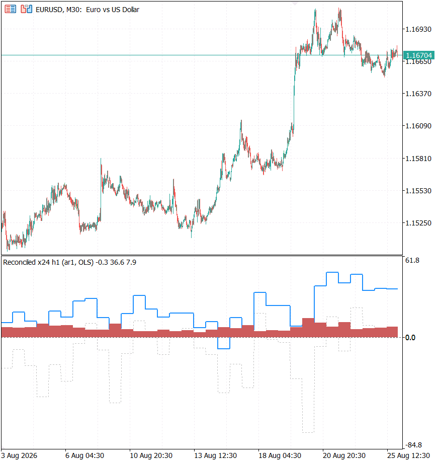
Fig. 6. ReconciledForecast on EURUSD H1, with the incoherence histogram below
Conclusion
We set out to replace a weighted vote with an estimator, and the estimator turned out to have more to say than the replacement itself.
- Coherence is a linear constraint, and cheap to impose. Timeframe aggregation and currency arithmetic become the same summing matrix, served by one engine. A third structure means filling in S; substituting your own models means editing BaseForecast.mqh, the only place a price series becomes a number.
- The guarantee does what the theorem says, and no more. On the timeframe hierarchy the orthogonal projection made no origin worse, 0 of 2,087. On the currency graph, whose bar closes satisfy the identity only to within 0.6 bp, it worsened 5.5% of hours and still cut pooled error by 0.48% at p below 0.0001.
- The gain tracks the contradiction. Sorted by base incoherence, the improvement runs monotonically from -5.2% to -35.2%. The buckets are whole-sample quantiles, so this is a diagnostic, not a trade, and it shows that the residue measures your procedure, not the market.
- Textbook MinT was a trap here. The sample covariance inflated error by 109% on sixty nodes, and by hundreds of percent on a shorter window, against 1.1% on twenty-one. It still got closer to the truth in its own metric at every origin: the failure is in the estimate of W, not in the projection. Shrinkage made it usable on the long window.
- The trace is not your objective. Reconciliation will sacrifice one node to help the rest. If you act on a single forecast, check that node: ours got 79% worse exactly when the hierarchy gained most.
That is the gap between what the method promises and what a trader usually wants. Reconciliation is an excellent way to improve a set of forecasts; it is not, without care, a way to improve the one you trade.
Getting the Source Code via MQL5 Algo Forge
All source files are attached to this article below, but the full repository is also available on MQL5 Algo Forge, the community's Git-based platform for sharing and collaborating on trading projects.
| File name | Description |
|---|---|
| MQL5\Include\Reconcile\ReconcileTypes.mqh | Shared enums and the dense linear algebra kernel: Cholesky with escalating ridge, triangular solves, SPD inverse and the Diebold-Mariano test |
| MQL5\Include\Reconcile\Shrinkage.mqh | Rolling store of base forecast errors, with sample, diagonal and Schaefer-Strimmer shrunk covariance estimates |
| MQL5\Include\Reconcile\Reconcile.mqh | CReconciler: the projection onto the coherent subspace, the five weighting schemes, reconciled covariance and the incoherence measure |
| MQL5\Include\Reconcile\Hierarchy.mqh | Both summing matrices, the union-find connectivity check, and the time-keyed multi-symbol bar loader |
| MQL5\Include\Reconcile\BaseForecast.mqh | Deliberately plain per-node base forecasters: last value, window mean and fitted AR(1) |
| MQL5\Scripts\Reconcile\Recon_Inspect.mq5 | Prints the summing matrix, the per-node reconciliation adjustment, the three projection invariants, and the raw triangle violations for the currency hierarchy |
| MQL5\Scripts\Reconcile\Recon_Evidence.mq5 | Walk-forward comparison of base forecasts against five weightings, per-level errors, Diebold-Mariano tests, the per-origin guarantee check and the incoherence bucket diagnostic |
| MQL5\Indicators\Reconcile\ReconciledForecast.mq5 | Base against reconciled forecast for one node of the temporal hierarchy, with the incoherence histogram |
Warning: All rights to these materials are reserved by MetaQuotes Ltd. Copying or reprinting of these materials in whole or in part is prohibited.
This article was written by a user of the site and reflects their personal views. MetaQuotes Ltd is not responsible for the accuracy of the information presented, nor for any consequences resulting from the use of the solutions, strategies or recommendations described.

 Features of Custom Indicators Creation
 Surrogate Data Testing: A Null Model for Any Statistic, and Why Shuffling Bars Is Not One
 Features of Experts Advisors
 Evolutionary Selection of LLM Agents in MetaTrader 5

- Free trading apps
- Over 8,000 signals for copying
- Economic news for exploring financial markets
You agree to website policy and terms of use