Online Portfolio Selection: A Provable Regret Bound, and the Cost That Eats It

Contents

• Introduction
• The wealth game, and what a regret bound promises
• The shared primitive: projection onto the simplex
• Follow the winner: EG and Cover's universal portfolio
• Follow the loser: PAMR and OLMAR
• The benchmark you are not allowed to trade
• Charging for the trading it implies
• Verification: three anchors of different strength
• What real markets say
• Does the gross advantage mean anything in the first place?
• Does regret per period actually shrink?
• Watching it on a chart, and putting it on an account
• Conclusion

Introduction

Most portfolio methods published for this platform start the same way. You collect returns, you build a covariance matrix, you feed it to an optimizer, and you get weights. The weakness is not the optimizer. It is that the matrix you built from the last 500 bars is not the matrix that governs the next 500, and the optimizer has no way of knowing that. Estimation error is the quiet tax on the whole family.

Online Portfolio Selection answers that differently. It estimates no statistical model: no covariance matrix, no return forecast, no distributional assumption. That is not the same as assuming nothing, and the mean reversion algorithms later in this article carry an explicit hypothesis about market structure along with a window, a threshold and a chosen basket. Each period you choose a portfolio, the market reveals what the prices did, your wealth multiplies by the dot product of the two, and you update. What replaces the model is a guarantee about regret: how far behind you finish against the best fixed portfolio somebody could have chosen if they had known the whole future in advance. Cover proved in 1991 that a specific algorithm keeps that gap growing slower than time itself, on any sequence of prices that meets the model's own technical conditions: price relatives strictly positive and bounded, so log wealth stays finite. Not on average, not under an assumption of normality, not for a stationary market. Within those conditions, any sequence.

That is a genuinely unusual kind of result in quantitative finance, and the paradigm is absent from this platform. The portfolio articles here are all batch estimation of one kind or another: Hierarchical Risk Parity clusters a correlation matrix, Markowitz with VaR optimizes against estimated moments, and Portfolio Optimization in Python and MQL5 fits its allocation to a sample. Every one of them estimates first. Nothing implements the online, regret-bounded family. Kelly sizing has been covered, and it is worth naming the difference up front. The best constant rebalanced portfolio in this article maximizes the same objective Kelly does, log wealth, but it is not a traded Kelly portfolio: Kelly sizes against a distribution you hold in advance, while this one is fitted to the sample after the fact and cannot be traded at all. The online algorithms sit in neither camp. They estimate no distribution, but they do carry hyperparameters and a structural assumption, which is a weaker claim than needing nothing.

This article builds the library and verifies it rigorously. Then it asks the question the theory does not answer. A regret bound applies to gross wealth, but trading costs reduce net wealth. The last third of this article is the measurement of what happens when you charge for the trading the guarantee implies, and that measurement is the reason to read it. The code blocks below are excerpts chosen to show the decisions; the complete files, with the class definitions, constants and error paths they rely on, are in the attached archive.

The wealth game, and what a regret bound promises

The setup is small enough to state completely. You have N assets. At period t you choose weights b_t that are non-negative and sum to one. The market then reveals price relatives x_t[i] = P_t[i] / P_(t-1)[i], and your wealth multiplies:

S_t = S_(t-1) * (b_t . x_t)

You see x_t, you update to b_(t+1), and it repeats. Total wealth after T periods is the product of every one of those dot products. Nothing has been assumed about how prices behave, beyond the two conditions the mathematics needs: every price relative is strictly positive, and the portfolio return b . x never reaches zero, or its logarithm is undefined. The library enforces the second with a floor, OLPS_WEALTH_FLOOR at 1e-12, on every b . x it takes a logarithm of. Real price data never reaches it. Degenerate data does, and what is being maximized there is a floored surrogate rather than log wealth itself, which is worth knowing before reading any claim of agreement with the theory.

The benchmark this family measures against is the constant rebalanced portfolio, or CRP: pick fixed weights and rebalance back to them every period. That sounds like a null strategy, and the reason it is not is the single most surprising fact in the field. Consider two assets. The first never moves. The second doubles, halves, doubles, halves. Both end exactly where they began, so buying and holding either one earns nothing. Now hold half of each and rebalance every period:

up period:             0.5 * 1.0 + 0.5 * 2.0 = 1.5
down period:           0.5 * 1.0 + 0.5 * 0.5 = 0.75
two periods together:  1.5 * 0.75            = 1.125

The rebalanced portfolio grows 12.5% every two periods out of two assets that go nowhere. Rebalancing forces you to sell what rose and buy what fell, and on an oscillating series that is a harvest. Over twenty periods it compounds to 1.125^10, which is 3.247321.

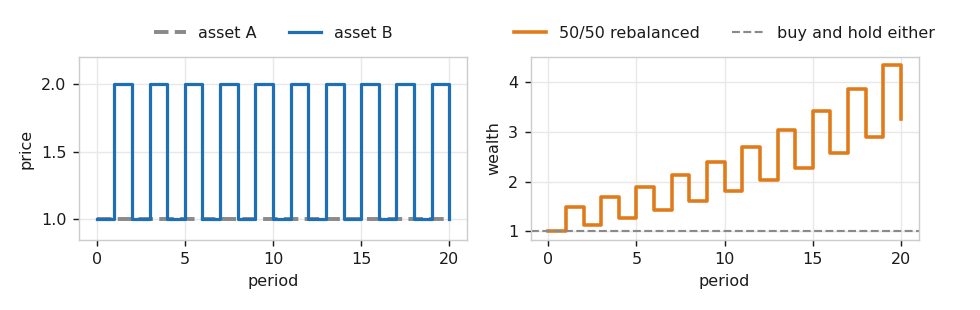
Fig. 1. Both assets end where they started, so the dashed line at 1.0 is what holding either one earns. The staircase is the same two assets held half and half and rebalanced every period

BCRP is the best constant rebalanced portfolio, chosen with hindsight. It is not a strategy, because computing it requires the future. It is the yardstick. Regret is the gap:

Regret_T = log(S_BCRP) - log(S_algorithm)

An algorithm is called universal when Regret_T divided by T goes to zero. Per period, you eventually stop losing ground to a portfolio chosen by someone who knew everything. That is the promise, and it comes with no distributional strings attached.

One thing to fix in your head now, because every measurement later in this article depends on it. BCRP bounds constant portfolios. It does not bound adaptive ones. An algorithm that changes its weights every period can and sometimes does finish ahead of BCRP, and for the mean reversion family that is the entire point. The invariant worth asserting is that no fixed portfolio beats BCRP, which is a test of the optimizer rather than of the theory.

The shared primitive: projection onto the simplex

Three of the five allocators here work the same way. PAMR and OLMAR add a step to the current weights, and the BCRP solver takes a gradient step, and each lands on a vector that is almost certainly not a portfolio: some component is negative, and the sum is not one. They then find the nearest point that is a portfolio. That nearest point operation is Euclidean projection onto the simplex. The other two never need it. EG takes a multiplicative step and renormalizes, which cannot leave the simplex, and Cover's universal portfolio only ever forms a convex mixture of portfolios it already holds. So projection is the primitive those three share, not a general operation of the whole family, and it is the piece worth getting exactly right.

The result is not an approximation and does not need an optimizer. There is a single threshold that, subtracted from every weight and then clipped at zero, produces the exact projection. Finding it takes one sort. This is Duchi et al. (2008), and the implementation follows the same early-break form the Python reference uses so the two agree bit for bit.

//+------------------------------------------------------------------+
//| Euclidean projection onto { b >= 0, sum b = 1 }                  |
//|                                                                  |
//|  Duchi et al. (2008). Subtracting one threshold from every       |
//|  weight and clipping at zero is the exact projection, not an     |
//|  approximation, and the sort is the entire cost.                 |
//+------------------------------------------------------------------+
void COLPSSimplex::Project(const double &v[], double &out[])
  {
   int m = ArraySize(v);
   ArrayResize(out, m);
   if(m == 0)
      return;
 
   double s[];
   ArrayResize(s, m);
   for(int i = 0; i < m; i++)
      s[i] = v[i];
   SortDesc(s, m);
 
   double tmpsum = 0.0;
   double tmax = 0.0;
   bool found = false;
 
   for(int i = 0; i < m - 1; i++)
     {
      tmpsum += s[i];
      tmax = (tmpsum - 1.0) / (double)(i + 1);
      if(tmax >= s[i + 1])
        {
         found = true;
         break;
        }
     }
 
   if(!found)
      tmax = (tmpsum + s[m - 1] - 1.0) / (double)m;
 
   for(int i = 0; i < m; i++)
      out[i] = MathMax(v[i] - tmax, 0.0);
  }

The loop walks the sorted weights accumulating a running sum, and at each position asks whether the threshold implied by keeping the top i+1 components would still leave the next component below it. The first position where that holds identifies how many components survive. Everything below the threshold is clipped away.

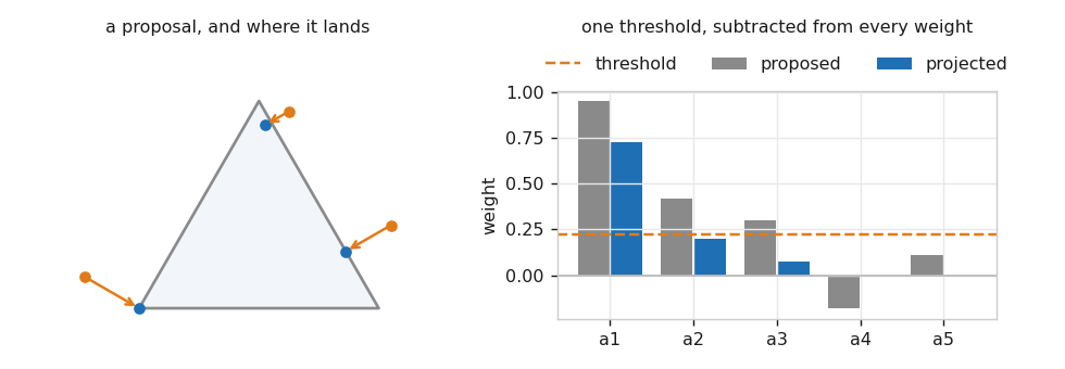
Fig. 2. For three assets the simplex is a triangle. 

That last point is what makes the projection more than a rescaling: it can drop an asset entirely, and that is what lets these algorithms concentrate.

The simplex is also long-only by construction. Weights are non-negative, so nothing built on this can short. That is a property of the method, not a limitation of this implementation, and it matters when you get to the expert.

Follow the winner: EG and Cover's universal portfolio

The literature splits into two families that move in opposite directions. The first increases weight on what has been performing. Exponentiated Gradient (Helmbold et al., 1998) is the clean representative: a multiplicative step along the gradient of log wealth.

//+------------------------------------------------------------------+
//| Reweight by exp(eta * x_i / (b.x)), then renormalize             |
//|                                                                  |
//|  The identity with UCRP is exact at eta = 0 only; at eta > 0 it  |
//|  is a limit, so the test runs eta = 1e-12 and matches UCRP to    |
//|  1e-6 rather than asserting equality.                            |
//+------------------------------------------------------------------+
void COLPSEg::Step(const double &b[], COLPSPanel &panel, const int t, double &out[])
  {
   double x[];
   panel.RelRow(t, x);
 
   double denom = MathMax(OLPSDot(b, x), OLPS_WEALTH_FLOOR);
   ArrayResize(out, m_n);
 
   double total = 0.0;
   for(int i = 0; i < m_n; i++)
     {
      out[i] = b[i] * MathExp(m_eta * x[i] / denom);
      total += out[i];
     }
 
   if(total <= 0.0)
     {
      m_simplex.Uniform(m_n, out);
      return;
     }
   for(int i = 0; i < m_n; i++)
      out[i] /= total;
  }

An asset's weight is multiplied by the exponential of its contribution to last period's return, scaled by a learning rate eta. Because the update is multiplicative and everything is renormalized, the result stays on the simplex without needing the projection at all. The comment box names a property worth having in a test. At eta = 0 every exponential is exactly one and EG is the uniform rebalanced portfolio identically; at any eta above zero that is a limit rather than an identity. The test suite exercises the limit at eta = 1e-12, where the two final wealths agree to within the 1e-6 the assertion demands.

Cover's Universal Portfolio is the algorithm the regret theorem is actually about, and its idea is startlingly direct: hold every constant rebalanced portfolio simultaneously, and weight them by the wealth each has earned so far. The exact version integrates over the whole simplex, and Cover's theorem is a statement about that integral. What a computer runs is a finite sample of portfolios, which is a different strategy rather than a noisier reading of the same one, and the bound does not transfer to it as stated. Keep the three apart from here on, because this section measures all three: the theorem, which belongs to the exact algorithm; the sampled implementation this library ships; and the empirical behavior of that implementation at 500 and at 16000 samples. The sampler matters too. Drawing n-1 uniforms, sorting them, and taking the gaps produces exactly Dirichlet(1,...,1), which is the uniform distribution on the simplex, with no rejection step. That makes the sampled portfolios reproducible from a seed, which is what lets the cross-check compare them for equality rather than for similarity.

//+------------------------------------------------------------------+
//| Compound every sampled portfolio, then re-mix                    |
//|                                                                  |
//|  Rescaling by the largest wealth keeps the sum finite over long  |
//|  histories. The mix depends only on ratios, so it changes no     |
//|  answer - without it the sum overflows on a few hundred bars.    |
//+------------------------------------------------------------------+
void COLPSUp::Step(const double &b[], COLPSPanel &panel, const int t, double &out[])
  {
   double x[];
   panel.RelRow(t, x);
 
   double biggest = 0.0;
   for(int j = 0; j < m_points; j++)
     {
      double g = 0.0;
      for(int i = 0; i < m_n; i++)
         g += m_w[j * m_n + i] * x[i];
      m_s[j] *= MathMax(g, OLPS_WEALTH_FLOOR);
      if(m_s[j] > biggest)
         biggest = m_s[j];
     }
 
   if(biggest > 0.0)
      for(int j = 0; j < m_points; j++)
         m_s[j] /= biggest;
 
   Mix(out);
  }

The portfolios themselves never move. Only their wealths do, and the portfolio actually held is their wealth-weighted average, which is what Mix forms. The rescaling by the largest wealth is the one line that is not in the textbook statement: over a few hundred bars the individual wealths spread across many orders of magnitude and the sum overflows, while the mix depends only on their ratios, so dividing them all by the largest changes no answer and keeps the arithmetic finite.

How many samples does that need? Sweep the count, run five seeds at every point, and use the spread as well as the mean. The spread is the part that answers the question.

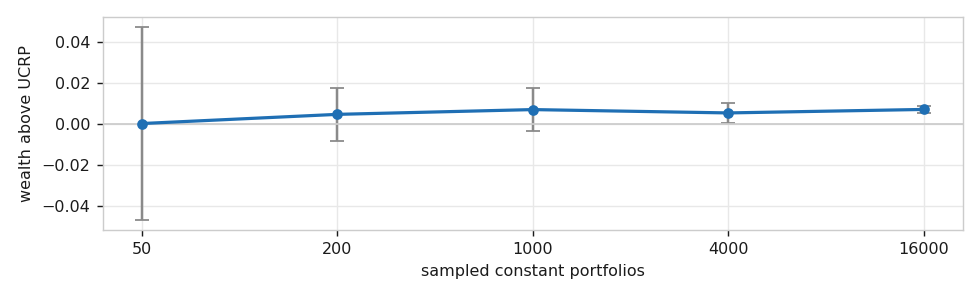
Fig. 3. Wealth above the uniform portfolio against the number of sampled portfolios, with one standard deviation across five seeds. Every bar overlaps every other, so the level is not resolved at all until the bars shrink

The point estimates are +0.000086, +0.004561, +0.006890, +0.005262 and +0.006961, and the standard deviation across seeds falls from 4.71e-02 to 1.85e-03, a factor of twenty-five. Those two rows only mean something read together. At 50 samples the standard error on the mean is 0.021, so that first estimate is equally consistent with the +0.007 the sweep settles on and with zero. Only at 16000 samples, where the standard error is 8.3e-04, is the advantage clearly separated from zero. Two things move at once when the count rises, and they should not be conflated. The strategy changes, because a 50-portfolio mixture and a 16000-portfolio mixture are different algorithms holding different weights; and the measurement sharpens, because the spread across seeds falls by that factor of twenty-five. What the error bars show is that across this range the second effect dominates the first: every interval overlaps every other, so the level is consistent with all of them. A single run at a low count is one draw from a distribution nearly seven times wider than the effect, and reading a trend off five such draws is reading noise.

Follow the loser: PAMR and OLMAR

The second family bets the opposite way: what just rose is about to give it back. PAMR (Li et al., 2012) stays completely still while the last period's portfolio return was below a threshold eps, and once it is above, moves the smallest distance that pushes the expected return back down to eps. OLMAR (Li and Hoi, 2012) reverts toward a moving average instead of toward the last period, which makes it the stronger of the two on real data and the one the library defaults to.

//+------------------------------------------------------------------+
//| Step toward the assets trading below their own average           |
//|                                                                  |
//|  Before the window exists the prediction is no change, so the    |
//|  step is a no-op. The reference instead feeds a normalized       |
//|  price level here, which depends on where its sample was cut.    |
//+------------------------------------------------------------------+
void COLPSOlmar::Step(const double &b[], COLPSPanel &panel, const int t, double &out[])
  {
   int last = t + 1;
 
   double xpred[];
   if(last < m_window)
     {
      ArrayResize(xpred, m_n);
      for(int i = 0; i < m_n; i++)
        xpred[i] = 1.0;
     }
   else
      Predict(panel, last, xpred);
 
   double xbar = 0.0;
   for(int i = 0; i < m_n; i++)
      xbar += xpred[i];
   xbar /= (double)m_n;
 
   double norm2 = 0.0;
   for(int i = 0; i < m_n; i++)
      norm2 += (xpred[i] - xbar) * (xpred[i] - xbar);
 
   double lam = 0.0;
   if(norm2 > 0.0)
      lam = MathMax(0.0, (m_eps - OLPSDot(b, xpred)) / norm2);
 
   double prop[];
   ArrayResize(prop, m_n);
   for(int i = 0; i < m_n; i++)
      prop[i] = b[i] + lam * (xpred[i] - xbar);
 
   m_simplex.Project(prop, out);
  }

The prediction is a moving average of the last few prices divided by the newest price, so an asset trading below its own average predicts a relative above one. The step direction is the excess of each prediction over the cross-sectional mean, and lam is the smallest multiplier that lifts the predicted portfolio return to eps. If every asset predicts the same thing, norm2 is zero, there is no relative information, and the correct step is none.

That warmup branch deserves a note, because it is where this implementation deliberately parts company with the Python reference. While there is not yet enough history for the moving average, the reference feeds a normalized price level into the slot that expects a price relative. Those are different quantities: a level says how far the asset has come since the sample began, and a relative says how far it moved since yesterday. The consequence is measurable rather than theoretical. Rerun the same prices but start ten rows later, and the reference's warmup weights can differ by up to 1.000. After the warmup, the two runs agree to 0.00e+00. Scaling the entire price panel changes nothing, which confirms it is the sample's start point and not its scale. This library predicts no change during warmup and therefore does not trade, and the cross-check compares after the warmup ends.

Important: PAMR's variant 0 in the reference divides by norm2 without a guard, so a period where every asset moved alike raises a division warning. The MQL5 version returns a zero step instead. The two agree on every other period, but that one line is a deliberate difference and not a porting error.

The benchmark you are not allowed to trade

BCRP is the maximizer of total log wealth over the simplex, given the whole history:

b_BCRP = argmax{ sum over t of log(b . x_t) : b >= 0, sum b = 1 }

That objective is concave, which is a gift: there are no bad local maxima for an ascent to get trapped in, so no restarts and no multi-start are needed. It does not follow that a finite run of one particular ascent has reached the maximum, and this one does not prove that it has. The library uses projected gradient ascent with a backtracking step, reusing the same projection PAMR and OLMAR use, and it stops on a gain tolerance rather than on a KKT residual or a bound on the duality gap. What that buys is a monotone sequence whose last point is the best one seen. The scipy comparison in the next section is an empirical check on that point, not a proof of its optimality.

//+------------------------------------------------------------------+
//| Projected gradient ascent with a backtracking step               |
//|                                                                  |
//|  Log wealth is CONCAVE on the simplex, so there are no bad local |
//|  maxima to restart away from. The stop is a gain tolerance and   |
//|  not a KKT residual, so this returns the best point a monotone   |
//|  ascent reached, not a certified global maximum.                 |
//+------------------------------------------------------------------+
double COLPSBcrp::Solve(COLPSPanel &panel, double &b[])
  {
   int T = panel.RelRows();
   int n = panel.Cols();
   m_used = 0;
 
   m_simplex.Uniform(n, b);
   if(T < 1)
      return(0.0);
 
   double f = LogWealth(b, panel);
   double step = 1.0 / (double)T;
 
   double grad[], prop[], cand[];
   ArrayResize(grad, n);
   ArrayResize(prop, n);
 
   for(int it = 0; it < m_iters; it++)
     {
      ArrayInitialize(grad, 0.0);
      for(int t = 0; t < T; t++)
        {
         double g = 0.0;
         for(int i = 0; i < n; i++)
           g += b[i] * panel.Rel(t, i);
         g = MathMax(g, OLPS_WEALTH_FLOOR);
         for(int i = 0; i < n; i++)
           grad[i] += panel.Rel(t, i) / g;
        }
 
      bool moved = false;
      double gain = 0.0;
      double trial = step;
 
      for(int k = 0; k < 60; k++)
        {
         for(int i = 0; i < n; i++)
           prop[i] = b[i] + trial * grad[i];
         m_simplex.Project(prop, cand);
 
         double fc = LogWealth(cand, panel);
         if(fc > f + 1.0e-15)
           {
            gain = fc - f;
            for(int i = 0; i < n; i++)
              b[i] = cand[i];
            f = fc;
            step = trial * 2.0;
            moved = true;
            break;
           }
         trial *= 0.5;
        }
 
      m_used++;
      if(!moved || gain < m_tol)
        break;
     }
 
   return(f);
  }

The inner loop halves the step until it finds one that strictly improves, and doubles the starting step on success so the search accelerates when the surface is smooth. On the eight-symbol basket used later it converges in 18 ascent steps (7.55 ms).

Cover's two-asset example gives this solver an exact target to hit. Maximizing log(1+p) + log(1-0.5p) over the weight p on the volatile asset differentiates to a single stationary point at p = 0.5, so the true BCRP is exactly 50/50 and its wealth is exactly 1.125^10. The library returns 0.500000 / 0.500000 and 3.247321. That is a closed form to check an optimizer against, which is rarer than it sounds.

Charging for the trading it implies

Here is where the theory and a trading account part company. Regret is defined on gross wealth. Every one of these algorithms produces a new set of weights every period, and moving to them costs spread and commission. Charging for that correctly turns on one detail that is easy to get backwards.

After you hold b through a period of relatives x, your weights are no longer b. The winners are now a larger share of the account than they were. The market has already done part of the rebalancing for you:

//+------------------------------------------------------------------+
//| Where a portfolio sits after one period, before rebalancing      |
//|                                                                  |
//|  Holding b through x leaves the weights at b*x/(b.x): winners    |
//|  are a bigger share than they were. Turnover must be charged     |
//|  against this, or rebalancing looks free.                        |
//+------------------------------------------------------------------+
void OLPSDrift(const double &b[], const double &x[], double &out[])
  {
   int n = ArraySize(b);
   ArrayResize(out, n);
   double denom = MathMax(OLPSDot(b, x), OLPS_WEALTH_FLOOR);
   for(int i = 0; i < n; i++)
      out[i] = b[i] * x[i] / denom;
  }

Turnover is the distance from that drifted portfolio to the new target, not from the previous target to the new one. Charge against the previous target and rebalancing looks free whenever the market happened to move you where you wanted to go. The wealth engine measures it the right way:

      double turn = 0.0;
      if(t == 0)
        {
         for(int i = 0; i < n; i++)
           turn += MathAbs(b[i]);
        }
      else
        {
         OLPSDrift(prevB, prevX, held);
         for(int i = 0; i < n; i++)
           turn += MathAbs(b[i] - held[i]);
        }
 
      double gross = MathMax(OLPSDot(b, x), OLPS_WEALTH_FLOOR);
      wealth *= gross * (1.0 - m_cost * turn);

The cost rate is charged per unit of traded weight. Moving 10% of the account from one asset to another gives a sum of absolute changes of 0.20, which is a 10% sale plus a 10% purchase, so the rate is a one-way cost and the round trip is counted correctly. Entry is charged once, at t = 0, where the whole book has to be established from nothing. A panel where nothing ever moves pays exactly 1.000 in total turnover, which the test suite asserts.

Verification: three anchors of different strength

The reference implementation for this field is the Python package universal-portfolios, and unlike several other reference libraries this one installs and runs on current Python. That makes the strongest level of checking an equality against published code rather than a statistical comparison. The verification is layered deliberately, because an anchor that agrees with everything proves nothing. One limit applies to the whole table below and is worth stating before it. Agreeing with published code to machine precision establishes that the port is faithful. It does not establish that either side is mathematically right, and a questionable convention in the reference would be reproduced rather than caught. The row that depends on nobody's code is the KKT check on the projection, and the BCRP row is one numerical optimizer agreeing with another.

Anchor	What it checks	Measured
Shared generator	MQL5 and Python draw the SAME sampled portfolios from one seed	0.000e+00 on the stream, the uniforms and the sampled portfolios
Published reference	EG, PAMR and OLMAR weight paths against universal-portfolios	worst 1.1e-12 over four cases; on real bars EG 9.4e-16 and PAMR 3.6e-15 over 398 rows, OLMAR 0.00e+00 over the 392 that follow its warmup
The definition	BCRP against scipy on the same concave objective	scipy never beats the MQL5 answer; worst gap -1.9e-13
Self-contained	Projection satisfies its own KKT conditions, no second implementation needed	worst residual 4.4e-16 over 40 cases

The generator is worth a sentence on its own. MQL5's ulong and Python's masked integers wrap identically, so a splitmix64 seed feeding an xorshift64* stream produces the same 64-bit words in both languages. Cover's universal portfolio draws its sampled portfolios from that stream, which is why the cross-check can demand exact equality on them instead of comparing distributions. The reference package cannot participate in that particular check, because its own sampler uses an unseeded generator, so its universal portfolio is not reproducible even against itself.

Each level prints its own pass and fail counts to the Experts log:

Level	What runs it	Result
Blueprint	python olps_prototype.py	34 PASS, 0 FAIL
Library	OLPS_Test_Core.mq5	31 PASS, 0 FAIL, 22 ms on an idle terminal and up to 38 with other charts running
Cross-check	OLPS_Export_ForCrosscheck.mq5, then python olps_crosscheck.py	57 PASS, 0 FAIL

The exporter writes to the terminal's common files folder, which is shared between terminals and is not the folder the cross-check sits in. Either copy olps_export.txt next to the script, or set the OLPS_EXPORT environment variable to the full path of that file, the file itself and not the folder holding it. Run it with neither and it prints the path it looked in and stops.

One assertion in that suite is worth singling out, because the obvious version of it is false. "No algorithm can beat BCRP" is not a theorem. BCRP bounds constant portfolios only, and an adaptive arm can finish ahead of it: on one of the random draws in this suite the mean reversion arm does exactly that, at a regret of -0.021781. What the suite asserts instead is the statement that is true, and it is a better test of the solver anyway: four hundred randomly sampled fixed portfolios, none of which beats it, worst shortfall -4.29e-02, reported rather than swallowed by a bare pass.

What real markets say

The market scan runs all five allocators on a real basket and then stress-tests the result. All results below use eight D1 symbols (EURUSDm, GBPUSDm, AUDUSDm, USDCADm, USDJPYm, XAUUSDm, XAGUSDm and US500m) with 1491 aligned bars from 2021.11.03. Read that line before any number under it: the basket is an intersection of calendars, and a symbol whose history has not finished downloading silently produces a smaller basket and different numbers. The allocators run at the library's own defaults throughout, and a result belongs to them: EG at eta 0.05, PAMR at eps 0.5 with C 500 and variant 0, OLMAR over a five-bar window at eps 10.0, and Cover's universal portfolio at 500 sampled portfolios.

Gross, the two mean reversion arms finish above the rebalanced baseline on these bars. PAMR finishes at 2.0321 and OLMAR at 1.7914 against the uniform portfolio's 1.5299, while EG at 1.5337 and Cover's universal portfolio at 1.5624 are barely distinguishable from it. None of the five reaches BCRP, which finishes at 2.9314 on the same bars. That shortfall is what regret measures, and the regret table later in this section recomputes it on every prefix rather than reusing this one number. One note on that 2.9314 before it gets compared to anything: it is a gross figure, and BCRP rebalances to fixed weights every period, so it would pay costs of its own. It is quoted gross because regret is defined gross, not as a claim that the number was attainable, and holding it beside a net column compares a hindsight yardstick with a traded outcome. Then you charge for the trading.

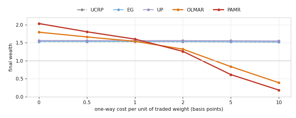
Fig. 4. The only two arms that beat the baseline gross are the only two destroyed by costs, and they cross the flat band between one and two basis points

That crossing is the finding. Below one basis point of one-way cost, PAMR and OLMAR are ahead. Above two, they are behind and falling. By five basis points PAMR has turned 2.0321 into 0.6152, which is a 70% destruction of the gross result.

Putting that crossing in trading units takes one step of care, because the rate is charged per unit of traded weight in one direction and is therefore a half-spread, not a round trip. One to two basis points is a two to four pip effective spread on a major. A raw-spread account beats that on EURUSD; a standard retail account paying spread plus commission does not; and the silver and index legs in this basket clear it on their own. A single rate is charged to all eight symbols here, even though their relative spreads differ by an order of magnitude, and FX, metals and indices also differ in commission, swap, session and contract specification. The crossing point is therefore a basket average, not a per-leg threshold. The model is a single linear rate on traded weight and nothing more: no bid and ask path, no slippage, no partial fills, no lot rounding, no currency conversion and no financing. None of that is charged anywhere in the sweep, so the basis-point axis is a simplified cost and not a live account's cost, and every number read off it inherits that simplification.

Arm	0 bp	1 bp	2 bp	5 bp	Turnover per bar
UCRP	1.5299	1.5286	1.5272	1.5231	0.0060
EG	1.5337	1.5324	1.5311	1.5271	0.0057
PAMR	2.0321	1.6003	1.2602	0.6152	1.6030
OLMAR	1.7914	1.5385	1.3213	0.8368	1.0211
UP	1.5624	1.5612	1.5599	1.5560	0.0055

The last column explains the rest of the table.

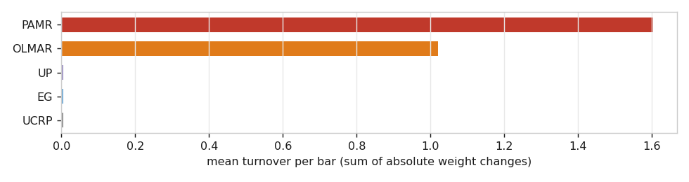
Fig. 5. PAMR turns the entire book over more than one and a half times per bar, and OLMAR once. The three arms that survive costs barely trade at all

PAMR's turnover of 1.6030 per bar means the sum of absolute weight changes exceeds 1.6 every single period. On a daily basket that is a complete portfolio replacement plus more, every day, for four years. The reason is its own threshold. PAMR sits still only while the portfolio's price relative is below eps, and eps ships at 0.5 while a portfolio of daily price relatives sits near 1.0, so on this data the passive branch never fires once. Moving eps toward 1.0 is what makes PAMR passive, and it is the single input that decides whether the algorithm is tradable at all.

The regret bound says nothing about any of this, because regret is defined on gross wealth and trading is free in the model. It says nothing about the ride either: charged at five basis points, PAMR's worst drawdown is 54.82% and OLMAR's 35.60%, against 11.02% for the baseline both of them were beating gross.

Does the gross advantage mean anything in the first place?

Before concluding that costs ruined a real edge, it is worth asking whether the edge existed. The null here is to shuffle whole rows of price relatives. Every asset keeps its own distribution of returns exactly, the cross section within a bar stays intact, and only the ordering in time is destroyed. If mean reversion is real, the algorithms should do worse on the shuffled version.

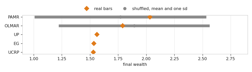
Fig. 6. The real result for both mean reversion arms sits comfortably inside the spread produced by shuffling the same bars. The three near-flat arms have no visible band because their wealth does not depend on order at all

Neither of them does worse on the shuffled bars. The p-value is the one-sided add-one estimate, p = (shuffles at or above the real result + 1) / (shuffles + 1), over 20 shuffles. PAMR reads 2.0321 against a null mean of 1.7699 with a standard deviation of 0.7630, giving p = 6/21 = 0.286. OLMAR reads 1.7914 against a null mean of 1.8922, so the shuffled version is on average better than the real data, at p = 10/21 = 0.476. Read the resolution before the values: at 20 shuffles the smallest p this test can return is 1/21 = 0.048, the grid moves in steps of 0.048, and a p near the middle of the range carries very little power. What a test this coarse can exclude is a large effect, not a small one.

The shuffle also destroys more than the signal it is aimed at. Volatility clustering and calendar effects go with the ordering too, so a null that kept clustering and reordered only direction, a block shuffle for instance, would be the stricter test. It is not run here. On the test that is run, the gross advantage of both arms sits inside what row shuffling produces by itself, which is not evidence of exploitable time structure.

Two details in that section are worth carrying away. The first is a free correctness check: BCRP sums log(b . x) over the whole history, and a sum does not care about order, so a correct shuffle must leave the benchmark exactly where it was. Measured worst gap across twenty shuffles is 7.47e-09, which is the ascent's own tolerance rather than true zero. Any larger gap would mean the shuffle had corrupted the data rather than reordered it.

The second is that some of those p-values are meaningless by construction, and the scan labels them rather than printing a number that looks like a test. The uniform rebalanced portfolio's wealth is a product of per-bar means, and a product does not care about order, so its null cannot move. Cover's universal portfolio is exactly invariant too, for a less obvious reason: the wealth-weighted mixture telescopes, so the portfolio's total wealth is simply the average of its sampled constant portfolios' wealths, and every one of those is a product as well. Both measured a null standard deviation of exactly zero over twenty shuffles, and EG is very nearly the same at 2.3e-05. Only PAMR and OLMAR have a live null at all.

Does regret per period actually shrink?

This is the question the title of this article raises, so it gets every arm rather than a representative one. Each column reruns the whole arm on a growing prefix of the same history and divides its shortfall against that prefix's own BCRP by the number of periods.

Arm	186	372	745	1117	1490
UCRP	0.00104	0.00032	0.00027	0.00037	0.00044
EG	0.00104	0.00032	0.00027	0.00037	0.00043
PAMR	0.00108	0.00013	0.00044	0.00026	0.00025
OLMAR	0.00092	0.00010	0.00028	0.00032	0.00033
UP	0.00103	0.00032	0.00027	0.00036	0.00042

Three things to read out of it. No row is monotone, and the wobble is not the algorithms being unstable: BCRP is refit on every prefix, so the target itself moves from column to column. The two mean reversion arms finish lowest, at 0.00025 and 0.00033 against the baseline's 0.00044, which is the direction an adaptive rule is supposed to move in. It is not more than a direction: PAMR's own row travels from 0.00108 to 0.00013 and back to 0.00044 across the columns, so the wobble within a row is four times the gap between rows in the last one, and the shuffled-bars null above has already put the same two arms' gross advantage inside what reordering the data produces by itself. And Cover's universal portfolio ends at 0.00042, indistinguishable from the fixed portfolio sitting above it. That row is not the theorem being tested either: the bound belongs to the exact integral over the simplex, and this column is a 500-portfolio sample of it.

That last row is not a refutation of the bound, and it should not be read as one. The uniform portfolio is a fixed portfolio and therefore not universal at all: its regret per period tends to a positive constant, because a better fixed portfolio genuinely exists. And 1490 periods is nowhere near long enough to watch a statement about the limit come true. What this table honestly shows is that the quantity is being measured correctly and that the horizon available on a real daily basket is far too short to see it converge.

Cost of the method itself is not a consideration. Over 1490 periods and eight assets, minimum of three runs, the uniform portfolio takes 0.56 ms, EG 1.11 ms, PAMR 1.52 ms and OLMAR 1.47 ms. Cover's universal portfolio at 500 sampled portfolios takes 36.68 ms, and it is the only one whose cost is worth thinking about, since it scales linearly with the sample count.

Three limits apply to everything in this section, and they are worth stating rather than leaving implied. It is one basket, one timeframe and one span, so the cost cliff is a property of this setup and not a universal threshold; a different basket composition would move it. Every arm runs at the library's defaults, and there is no sensitivity sweep over PAMR's eps, OLMAR's window and eps or EG's eta, which is the weakest point of the three, because the section itself shows PAMR's eps to be the input that decides whether the algorithm is tradable. And there is no out-of-sample or walk-forward split anywhere in it: every number above is in sample on the same 1491 bars. The section describes what those bars did and makes no claim about what the next ones will do.

Watching it on a chart, and putting it on an account

The indicator plots the decision-relevant quantity rather than the decision. It draws three wealth curves in a subwindow: the selected allocator net of costs, the uniform rebalanced baseline net of the same costs, and BCRP for scale. A panel on the main chart carries the basket line, the cost being charged, per-arm turnover and drawdown, and the current target weights as a small bar meter.

Two implementation notes, both easy to get wrong. A custom indicator cannot call Sleep, and one created through iCustom never receives a timer event, so the usual patterns for waiting on history do not work. Multi-symbol history also arrives asynchronously, so the first call for a symbol that is not in Market Watch returns nothing at all. The data layer selects each symbol before requesting it, which is what makes the terminal start providing it, and reports the symbols still pending by name rather than quietly building a smaller basket. Returning 0 from OnCalculate asks MetaTrader 5 to call again, which works on a live market and does nothing on a closed one, since no tick ever arrives to trigger the retry.

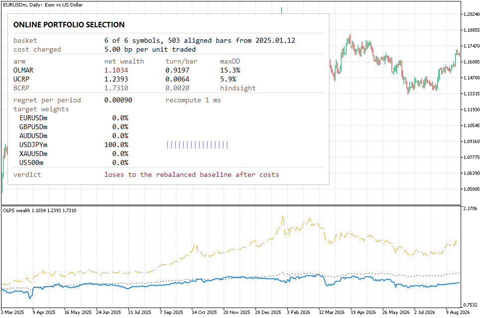
Fig. 7. OLMAR on a six-symbol basket, EURUSDm D1, charged at five basis points, plotting the newest 465 of the 503 bars the basket aligns on. Blue is the algorithm net of costs, dotted grey the rebalanced baseline net of the same costs, dashed orange the hindsight benchmark

That panel is the whole article in miniature, on a different basket and a different period from the scan. OLMAR finishes at 1.1022 against the baseline's 1.2398, so the verdict line says it loses after costs, and the turnover column says why: 0.9197 per bar against 0.0064, a factor of 144. Its worst drawdown is 15.3% against 5.9%. The target weights are the other thing to look at, because the projection has put the entire book into one leg and left the other five at zero. That is the earlier point about the simplex arriving on real data: the projection does not rescale, it drops assets.

The expert is a demonstration of how the reading is consumed, not a trading system, and no edge is claimed for it. It reloads the basket on every bar, runs the chosen allocator, and rebalances only when the distance from the book it actually holds to the new target exceeds a threshold. That gate exists because of the cost measurement above, and it is the one design decision in the expert that comes from evidence rather than convention.

Three things about running a multi-asset allocator on a real account are worth stating plainly, because none of them appear anywhere in the theory. The legs do not share a trading session, so a basket rebalanced on one symbol's bar routinely meets a closed market on another and comes back partial. A leg whose target rounds below the minimum lot is not an allocation of zero; it is an allocation the account is too small to express. One minimum lot of an FX major is roughly 1080 of notional, so a 10000 account spread over six symbols at half exposure cannot express any leg at all. And the turnover gate has to measure distance from the positions actually held, not from the weights last requested, or a constant-weight allocator concludes it never needs to trade and quietly becomes buy and hold.

Run with a baseline arm beside it, which is the only way the result is readable at all. The pair below is an illustration of what execution does to an account rather than a strict comparison of two strategies, for the reason given under the table. Both arms use deposit 100000, EURUSDm D1 from 2022.01.03 to 2026.08.01, a minimum turnover of 0.15 and half the equity allocated. The basket here is six symbols rather than the scan's eight, EURUSDm, GBPUSDm, AUDUSDm, USDJPYm, XAUUSDm and US500m, because every leg has to be tradable on the account and not merely present in the price panel:

Arm	Trades	Net	Profit factor	Balance drawdown	Rebalances
UCRP baseline	14	+6918.03	7.32	0.90%	5
OLMAR	669	-1176.07	0.99	14.98%	706

The allocator rebalances 141 times more often and turns a positive result into a negative one. That is the cost cliff showing up in a profit-and-loss statement instead of a table. Read it as execution reaching an account, and not as a measured difference between the two strategies: the arms are not looking at the same sample, because an arm that trades less is flat more often and reaches its decision point a different number of times, so the table cannot be a strict arm-to-arm comparison. The path independent evidence is the cost sweep in Fig. 4, not this pair.

Conclusion

Online Portfolio Selection delivers exactly what it promises and nothing more. The regret bound is real, it holds without any distributional assumption as long as price relatives stay positive and bounded, and the library reproduces the published reference implementation to machine precision, which establishes the port rather than the mathematics. What the bound does not cover is the cost of the trading it implies, and on this basket that cost is decisive: the crossing point sits between one and two basis points of one-way cost, which is a two to four pip effective spread on a major and which the metal and index legs of this basket clear on their own. The two algorithms that finish above a plain rebalanced portfolio gross here are precisely the two that cannot survive being charged, and neither of them clears a null built by shuffling the same bars into a different order. That makes their gross result an observation about this sample, at these defaults, over this span, and not evidence of an edge.

The honest summary is that this is a descriptive tool and a piece of theory worth understanding, not an edge. Regret is not profit and loss, and the distance between the two is measurable.

What the attached code gives you:

• A complete from-scratch library: exact simplex projection, uniform simplex sampling from a reproducible generator, five allocators (uniform CRP, EG, Cover's universal portfolio, PAMR, OLMAR), a BCRP solver by projected gradient ascent, and a wealth engine with a drift-aware transaction cost model.
• A multi-symbol data layer that intersects trading calendars, scores coverage over the shared span, and names the symbols it dropped or is still waiting for.
• A test script covering the generator, the projection, the sampler, Cover's analytic example and the per-algorithm invariants, plus an exporter and a Python cross-check that compares against universal-portfolios, against scipy, and against the definition.
• A market scan that reports the cost cliff, the shuffled-bars null, the regret decay and the per-arm timings on any basket you point it at.
• An indicator that plots net wealth against the rebalanced baseline, and a demonstration expert with a turnover gate and a control arm.

#	Filename	Type	Description
1	OLPS.mqh	Include	Facade: load a basket or a matrix, run an allocator, report regret and normalized regret
2	OLPSAlgo.mqh	Include	The Step interface every allocator implements, the uniform and fixed CRPs, dot product and portfolio drift
3	OLPSBenchmark.mqh	Include	Best constant rebalanced portfolio by projected gradient ascent on a concave objective
4	OLPSData.mqh	Include	Price panel and the multi-symbol loader: calendar intersection, coverage over the shared span, pending and dropped symbols named
5	OLPSLoser.mqh	Include	Follow the loser: PAMR and OLMAR mean reversion
6	OLPSPanel.mqh	Include	Panel geometry and glyph metrics, shared so a width budget and the check on it are one formula
7	OLPSRandom.mqh	Include	splitmix64 seeding into xorshift64*, matched bit for bit to the Python side
8	OLPSSimplex.mqh	Include	Exact Euclidean projection onto the simplex and uniform sampling from it
9	OLPSWealth.mqh	Include	The wealth game: wealth path, turnover, drawdown and the drift-aware cost model
10	OLPSWinner.mqh	Include	Follow the winner: Exponentiated Gradient and Cover's universal portfolio
11	OLPS_Test_Core.mq5	Script	Generator conformance, projection and sampler checks, Cover's analytic case, per-algorithm invariants and the cost model
12	OLPS_Export_ForCrosscheck.mq5	Script	Dumps the whole pipeline at full double precision for the Python cross-check
13	OLPS_Scan_Market.mq5	Script	Real baskets: the cost cliff, regret decay, the shuffled-bars null, the sample-count sweep and timings
14	OLPS_Allocation.mq5	Indicator	Net wealth against the rebalanced baseline and BCRP, with an allocation panel
15	OLPS_Rebalance_EA.mq5	Expert	Demonstration only: an online allocator behind a turnover gate, long-only, no profit claimed
16	olps_prototype.py	Python	The blueprint the MQL5 port follows statement for statement, with its own oracles
17	olps_crosscheck.py	Python	Cross-check runner: equality against the shared generator, the published reference, and the definition
18	MQL5.zip	Archive	Archive with all project files in their subfolders; unpack it into the terminal data directory and every file lands in its required location