Neural Networks in Trading: From Transformers to Spiking Neurons (Conclusion)

Introduction

Financial markets can be compared to a vast ocean, where the waves rise and fall every second. Sometimes the sea is calm and predictable; sometimes it rages and threatens to capsize a ship; and at other times, it appears deceptively smooth, hiding powerful currents beneath the surface. A trader in this ocean is like a skipper who must discern not every ripple on the water, but the very gust of wind that can set the movement in the right direction. A mistaken perception or misinterpretation of signals — and the ship goes down. This metaphor captures the very essence of the search for effective analytical tools. What matters is not the quantity of information, but its quality — the ability to make sense of the chaos.

This is exactly where the SpikingBrain framework opens up new horizons. It is based on the principles of event-driven processing. The system does not respond to a continuous stream of data, but only to those pulses that carry genuine meaning. For a trader, this means one thing: the model does not drown in a sea of market noise, but learns to pick up genuine signals capable of changing the course of trading.

In practical financial-market applications, this offers a number of advantages. First, computational costs are reduced, which is particularly important when working with high-frequency data. The model becomes lighter and faster, and it can be easily integrated into trading platforms without the risk of overloading the system. Second, noise resistance increases, which allows for clearer trading signals and reduces the likelihood of false entries. And finally, third, SpikingBrain enables adaptive response—the model’s ability to quickly readjust when the market unexpectedly changes direction.

The SpikingBrain framework is interesting not only for its philosophy of event-driven perception, but also for its architecture, which turns that philosophy into a practical tool. It is based on the idea of representing a data stream as a series of discrete pulses— a kind of spike. Each such pulse does not occur continuously, but only when an event occurs that disrupts the previous equilibrium. This makes it possible to shift from continuous analysis to working with compact yet information-rich data points.

The SpikingBrain architecture consists of several key modules, each responsible for its own aspect of market perception. The first thing that stands out is the spiking neurons with an adaptive threshold. They react only to events that go beyond the ordinary. The activation threshold changes dynamically depending on how the data behaves, making the model more sensitive or, conversely, filtering out minor fluctuations.

The second fundamental element is the attention module. Classical transformers are known for their ability to handle context. But this power comes at a high price. The longer the sequence, the more computationally intensive the calculations become. SpikingBrain solves this problem differently. It uses linear attention and a sliding-window strategy. In more complex versions, a hybrid approach is used, in which different types of attention work together. This allows the model to process long time series of prices and volumes without incurring exorbitant costs, while still maintaining the ability to see the big picture.

The Mixture of Experts mechanism plays a special role. In the version with the extended architecture, not all of the model's blocks operate simultaneously. Only those that are needed in a given situation are activated. Essentially, this reflects the trader's own strategy: trading in a measured way under normal conditions, but acting with particular focus during strong market moves.

But perhaps SpikingBrain's most elegant solution is its system for encoding events as spikes. The raw data is converted into a series of pulses, where each spike reflects not just the fact that the price has changed, but the significance of that change. The frequency and intensity of spikes become a kind of language through which the model describes the market. If the market movement is weak, the signal is infrequent and quiet. If the market erupts, the spikes turn into a loud peal of bells, and the system responds instantly.

Consequently, SpikingBrain is not just a set of mathematical tricks, but an attempt to build a model that thinks in terms of events. It can listen to the market. And that is precisely why its architecture deserves careful study, especially in the context of its application in financial markets.

The author’s visualization of the SpikingBrain framework is shown below.

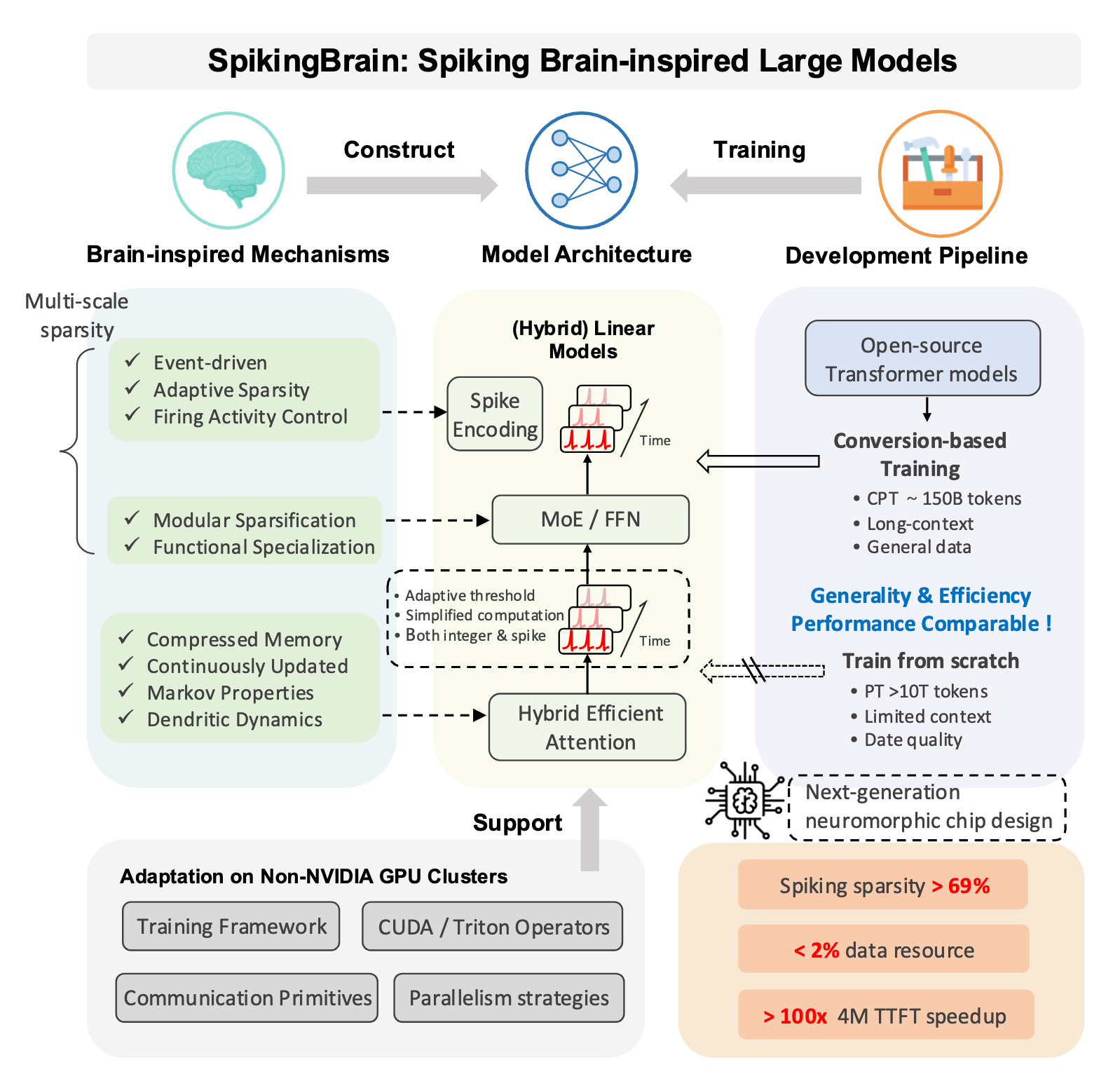
In science and technology, every architecture remains merely a diagram on paper until its lines and blocks come to life in a specific implementation. That is exactly why we are structuring our discussion of SpikingBrain in a step-by-step manner. Step by step, so that ideas don't just hang in the air but are transformed into practical tools for analysis. The architecture we discussed above sets the direction and outlines the structural framework. But any design only becomes meaningful when its components become part of practical work, and its theoretical modules become part of code that responds to the market flow.

Our journey began with our first encounter with SpikingBrain. First, we examined the framework authors’ ideas and tried to explain them through the lens of financial markets. Where the researchers' original text sounded academic, we looked for practical meaning. Essentially, it was laying the groundwork. We outlined the prospects and showed that SpikingBrain has the potential to go beyond pure theory.

Next, we showed how the ideas of event logic can be translated into code, and took an important step — we taught the model to convert a continuous stream of numbers into discrete spikes. The key element here was threshold-based signal conversion. A neuron remains silent until the value reaches a critical threshold, and only then does it fire a brief pulse. This approach immediately separated noise from truly significant changes and allowed us to look at prices from a different perspective. However, to prevent this mechanism from turning into a dead end, we added a learning capability—we made the thresholds adaptive and ensured that gradients could propagate even through silent neurons. As a result, the network gained the ability to adapt to the market over time, rather than remaining static.

However, we took it a step further and developed these ideas into a fully-fledged architecture. The key components responsible for keeping the system running came to the forefront. We integrated spiking transformations into the familiar layer structure and demonstrated how they can coexist with convolutional blocks and other classic neural network elements. Implementing this in MQL5 required careful consideration of memory and computing resources. Neurons must not fire simultaneously; otherwise, the very essence of the event-based approach is lost. That is why we designed a mechanism in which a significant portion of the neurons remains silent, while computational resources are concentrated where market movement is actually occurring. Essentially, we have laid the groundwork for SpikingBrain to integrate seamlessly into the trading ecosystem without disrupting the existing architecture, but rather by enriching it with a new, event-driven dimension.

Sparse Attention Module

We continue our journey from the general philosophy of event-driven systems to the concrete implementation of the proposed architecture. We descend from the heights of schematics straight onto the ship’s deck — into the code and execution logic. Earlier, we explained why SpikingBrain views the market as a chain of meaningful episodes and outlined the first practical steps for converting continuous activations into spikes. This naturally raises the question: how should this event-driven logic behave where local attention windows traditionally operate? What changes will be needed for local attention to operate in the spirit of spikes and withstand the onslaught of market noise?

The framework’s authors propose a shifted window, but the market is fickle. The distance between important bursts is dynamic, and noise usually fills the windows more densely than we would like, so we choose a different path — we preserve the sparse attention logic based on graphons. But we build it in a way that respects the very essence of spikes — asynchrony, adaptive thresholds, and the informational value of a neuron’s silence. We are talking about a reimplementation of the CNeuronSparseGraphAttention module — one that does not simply copy the previous implementation, but represents its evolution. CNeuronSpikeSparseAttention is our vigilant guardian of attention, adapted to the rhythm of the market and the language of spikes.

class CNeuronSpikeSparseAttention   :  public CNeuronSpikeConv
  {
protected:
   CNeuronConvOCL       cValue;
   CNeuronGraphons      cGraphs;
   CNeuronSparseSoftMax cScores;
   CNeuronBaseOCL       cAttention;
   //---
   virtual bool      feedForward(CNeuronBaseOCL *NeuronOCL) override;
   virtual bool      updateInputWeights(CNeuronBaseOCL *NeuronOCL) override;
   virtual bool      calcInputGradients(CNeuronBaseOCL *NeuronOCL) override;

public:
                     CNeuronSpikeSparseAttention(void) {};
                    ~CNeuronSpikeSparseAttention(void) {};
   //---
   virtual bool      Init(uint numOutputs, uint myIndex, COpenCLMy *open_cl,
                          uint units, uint window, uint experts, float dropout,
                          uint emb_dimension, uint sparse_dimension,
                          ENUM_OPTIMIZATION optimization_type, uint batch);
   //---
   virtual int       Type(void) override const   {  return defNeuronSpikeSparseAttention;   }
   //--- Methods for Working with Files
   virtual bool      Save(int const file_handle) override;
   virtual bool      Load(int const file_handle) override;
   //---
   virtual bool      WeightsUpdate(CNeuronBaseOCL *source, float tau) override;
   virtual void      SetOpenCL(COpenCLMy *obj) override;
   virtual void      TrainMode(bool flag) override;
  };

First and foremost, it is worth noting that the new object inherits from CNeuronSpikeConv — our mechanism for converting a continuous signal into spikes. That alone says a lot about the class's purpose. It does not reinvent spikes; it continues to process them properly. Inheritance ensures that the basic convolution logic and primary event encoding are inherited, while in the descendant class we focus exclusively on spike-based attention logic.

At first glance, the class body reveals a familiar set of internal objects: cValue, cGraphs, cScores, and cAttention. Their names are familiar — but what matters is that there are fewer of them than in the original implementation. We deliberately abandoned the residual-connection backbone and the separate FeedForward module. The reason is simple, and it is the same one we already mentioned when working with gated linear attention: in the event-driven paradigm, extra paths diffuse the pulse and lead to redundant computations. Instead, the residual path and the shared FFN are at the block level, where the results from different attention branches are aggregated and where it makes sense to align and amplify the signal once.

I would like to point out an important design detail. All internal objects are declared statically as class members. This allows the constructor and destructor to remain empty — initialization is moved to a separate Init method.

bool CNeuronSpikeSparseAttention::Init(uint numOutputs, uint myIndex, COpenCLMy *open_cl,
                                       uint units, uint window, uint experts, float dropout,
                                       uint emb_dimension, uint sparse_dimension,
                                       ENUM_OPTIMIZATION optimization_type, uint batch)
  {
   if(!CNeuronSpikeConv::Init(numOutputs, myIndex, open_cl, window, window, window,
                              units, 1, optimization_type, batch))
      return false;
   activation = None;

The Init method is the act of preparing the module for real market operation. The method signature contains everything needed to control the dimensions and behavior of sparse attention. Inside the method, we first delegate part of the initialization to the parent class to preserve compatibility with the spike encoder.

Next comes the sequential initialization of the internal modules. cValue is the first to take on the function of collecting the local representation — this is a convolution that prepares the V values for subsequent weighting.

   int index = 0;
   if(!cValue.Init(0, index, OpenCL, window, window, window, units, 1, optimization, iBatch))
      return false;
   cValue.SetActivationFunction(None);

Note that we immediately remove the activation from cValue. The reason is practical: spiking representations already carry nonlinearity and sparsity, and any additional pointwise activation at this stage only blurs the impulse. We need raw V vectors so that attention can correctly weight the contribution of each spike.

Next, the mixture of graphons, cGraphs, is initialized — this is the core of our sparsity. It studies the structure of the data, taking into account temporal distances, volumes, and spike density.

   index++;
   if(!cGraphs.Init(0, index, OpenCL, units, window, emb_dimension, experts, dropout, optimization, iBatch))
      return false;

cScores is our Sparse SoftMax. It takes the data structure proposed by the graphons and focuses only on the most significant neighbors, thereby creating sparsity in local attention. This approach reduces computational complexity to a level close to that of window-based attention while preserving flexibility — the window itself is dynamic and depends on current activity and spike statistics.

   index++;
   if(!cScores.Init(0, index, OpenCL, units, units, sparse_dimension, optimization, iBatch))
      return false;

cAttention accumulates the final result α·V.

   index++;
   if(!cAttention.Init(0, index, OpenCL, Neurons(), optimization, iBatch))
      return false;
   cAttention.SetActivationFunction(None);
//---
   return true;
  }

The practical significance of all these decisions is clear — we eliminate the redundant elements in advance because, in spiking logic, they more often get in the way than help. We keep only those elements that actually affect impulse selection. We organize memory so that the OpenCL kernel works with compact, compressed structures. This provides gains in latency and power consumption — two critical metrics for real-time trading.

We move from the initialization level directly to execution. The feedForward method is the very working routine where theory meets data. The algorithm is simple in structure and expressive in meaning. Nothing extra. Everything is aimed at one thing: the resulting output should reflect important spike pulses, not noise.

bool CNeuronSpikeSparseAttention::feedForward(CNeuronBaseOCL *NeuronOCL)
  {
   if(!cValue.FeedForward(NeuronOCL))
      return false;

First, the forward pass method of the cValue object is called. This is a convolutional stage that collects local features and forms the value matrix V. Here, we prepare what will be weighted by attention.

Next, graphon masks, a list of neighbors, and their relative weights are generated. The mask represents not a static window, but a dynamic neighborhood that depends on time, volume, and spike density. In this step, we decide exactly what to compare the analyzed position against.

   if(!cGraphs.FeedForward(NeuronOCL))
      return false;
   if(!cScores.FeedForward(cGraphs.AsObject()))
      return false;

cScores is used to obtain a sparse attention weight matrix from the generated graphons. In practice, cScores produces two key artifacts: compact indexes (neighbor lists) and an array of weights for each position–neighbor pair.

The key computational step is SparseMatMul. This function multiplies a sparse matrix of weights (scores) by a dense matrix of values V. The result is a dense attention matrix with continuous values.

   if(!SparseMatMul(cScores.GetIndexes(), cScores.getOutput(), cValue.getOutput(),
                    cAttention.getOutput(), cScores.Heads(), cScores.DimensionOut(),
                    cValue.GetUnits(), cValue.GetFilters()))
      return false;
//---
   return CNeuronSpikeConv::feedForward(cAttention.AsObject());
  }

The forward pass algorithm concludes with a call to the method of the same name in the parent class. This is a return to spike space. We pass the aggregated attention vector on to the spike encoding system. Here, thresholding and spike-generation mechanisms will be applied, and the module output will be prepared for merging at the upper level of the attention block.

Overall, feedForward is a synchronization node between the sparse logic of the graphon and spike encoding. It carefully translates the dynamic, local context into dense attention representations and returns them to the world of spikes.

I suggest you familiarize yourself with the backward-pass algorithms on your own. All details, including the complete class code and the implementation of each method, are provided in the attachment.

Mixture of Experts Variant

Now that the attention modules have been implemented, we will move on to building the Mixture of Experts module. We have encountered similar constructs in previous articles, but none of them was free of compromises. Striking a balance between computational efficiency and model expressiveness has always been a challenge. The spiking architecture paradigm adds its own distinctive features: neuron silence, sparse signals, and the dynamic activity of experts make the task even more nuanced. Therefore, within this work, we are creating a new object that takes these realities into account.

Once again, the issue of conserving computational resources and ensuring effective parallel operation of the experts comes to the forefront. The complexity is compounded by the fact that each element in the sequence may involve its own set of experts. And the standard approach — where each expert has its own input — quickly leads to redundant calculations.

To understand how to get around this, let's take a look at the author’s visualization of the MoE block.

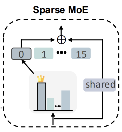
The experts' outputs are simply summed. And this presents an important opportunity for optimization. The same dataset is fed to all active experts. From a mathematical standpoint, this allows us to factor out the input and, instead of performing multiple separate projections, perform a single linear projection using the sum of the experts' parameters. This technique preserves the correctness of the calculations while significantly reducing the load on memory and the processor, which is especially important when working with long time series of financial instruments and high data update rates.

As a result, we get an efficient yet expressive MoE module that fits the philosophy of the spiking architecture and is ready to work with parallel streams of attention and market signals.

We implement the proposed approach as a new class called CNeuronMoEConv. This is a full-fledged module that integrates neatly into the spiking architecture and ensures efficient load distribution among the experts. The class inherits from the base CNeuronBaseOCL class, which allows it to operate in a unified OpenCL context alongside the other layers and interact easily with other modules.

class CNeuronMoEConv   :  public CNeuronBaseOCL
  {
protected:
   CLayer            acProbability;
   CParams           cExperts;
   CNeuronBaseOCL    cWeightsConv;
   //---
   virtual bool      feedForward(CNeuronBaseOCL *NeuronOCL) override;
   virtual bool      updateInputWeights(CNeuronBaseOCL *NeuronOCL) override;
   virtual bool      calcInputGradients(CNeuronBaseOCL *NeuronOCL) override;

public:
                     CNeuronMoEConv(void) {};
                    ~CNeuronMoEConv(void) {};
   virtual bool      Init(uint numOutputs, uint myIndex, COpenCLMy *open_cl,
                          uint units, uint window, uint window_out,
                          uint experts, float dropout, uint topK,
                          ENUM_OPTIMIZATION optimization_type, uint batch);
   //---
   virtual int       Type(void) override const   {  return defNeuronMoEConv;   }
   //--- Methods for working with files
   virtual bool      Save(int const file_handle) override;
   virtual bool      Load(int const file_handle) override;
   //---
   virtual bool      WeightsUpdate(CNeuronBaseOCL *source, float tau) override;
   virtual void      SetOpenCL(COpenCLMy *obj) override;
   virtual void      TrainMode(bool flag) override;
  };

Several key components are defined within the class. acProbability is responsible for the probabilistic distribution of expert activity, specifying which experts will participate in processing each element of the sequence. cExperts stores the parameters of all experts, which together form the model’s rich functional set. cWeightsConv is used to form the aggregate parameters of the active experts. This is where the idea of factoring out the input, mentioned earlier, is put into practice. This technique significantly reduces the number of computations and cuts memory usage without compromising the model's expressiveness.

A new object is initialized in the Init method, which carefully prepares all internal components and ensures that the layer functions correctly.

bool CNeuronMoEConv::Init(uint numOutputs, uint myIndex, COpenCLMy *open_cl,
                          uint units, uint window, uint window_out,
                          uint experts, float dropout, uint topK,
                          ENUM_OPTIMIZATION optimization_type, uint batch)
  {
   if(!CNeuronBaseOCL::Init(numOutputs, myIndex, open_cl, units * window_out, optimization_type, batch))
      return false;

First, the base initialization of the parent class is called.

Next, the key elements of the module are created and configured one by one. First, a chain is created to calculate expert activation probabilities: acProbability.

//---
   int index = 0;
//---
   CNeuronConvOCL       *conv    = NULL;
   CNeuronDropoutOCL    *dout    = NULL;
   CNeuronSparseSoftMax *softmax = NULL;
//--- Probability
   acProbability.Clear();
   acProbability.SetOpenCL(OpenCL);
   index++;
   conv = new CNeuronConvOCL();
   if(!conv ||
      !conv.Init(experts, index, OpenCL, window, window, 2 * experts, units, 1, optimization, iBatch) ||
      !acProbability.Add(conv))
     {
      DeleteObj(conv);
      return false;
     }
   conv.SetActivationFunction(SoftPlus);
   index++;
   conv = new CNeuronConvOCL();
   if(!conv ||
      !conv.Init(experts, index, OpenCL, 2 * experts, 2 * experts, experts, units, 1, optimization, iBatch) ||
      !acProbability.Add(conv))
     {
      DeleteObj(conv);
      return false;
     }
   conv.SetActivationFunction(SoftPlus);
   index++;
   dout = new CNeuronDropoutOCL();
   if(!dout ||
      !dout.Init(0, index, OpenCL, conv.Neurons(), dropout, optimization, iBatch) ||
      !acProbability.Add(dout))
     {
      DeleteObj(dout);
      return false;
     }
   index++;
   softmax = new CNeuronSparseSoftMax;
   if(!softmax ||
      !softmax.Init(0, index, OpenCL, units, experts, topK, optimization, iBatch) ||
      !acProbability.Add(softmax))
     {
      DeleteObj(softmax);
      return false;
     }
   softmax.SetHeads(units);

Here, a sequence of two convolutional layers is created, with SoftPlus activation between them. This approach ensures a smooth and stable distribution of values, which is particularly important when working with dynamic financial signals, where sharp spikes and noise can easily overwhelm the model. Convolutional layers generate expert relevance distributions for each element in the sequence, assessing which expert is most relevant at any given moment. The chain concludes with a sparse SoftMax function object, which selects a specified number of the most significant experts and assigns a significance coefficient to each one, allowing the model to focus on truly important market signals while ignoring noise and insignificant patterns.

Adding a Dropout layer before SoftMax regulates the random deactivation of elements, preventing overfitting and improving the model's resilience to market noise.

At the same time, the cExperts object is initialized; it stores the parameters of all experts, combining them into a single space.

   index++;
   if(!cExperts.Init(0, index, OpenCL, window * window_out * experts, optimization, iBatch))
      return false;
   index++;
   if(!cWeightsConv.Init(0, index, OpenCL, window * window_out * units, optimization, iBatch))
      return false;
//---
   return true;
  }

The cWeightsConv object serves as an aggregate set of parameters for active experts.

Each step in the initialization of internal components is accompanied by a check to verify that the operations were performed successfully. If the operation fails, the object is deleted, and the method returns false. This ensures the reliability and predictability of the layer's operation, even with complex combinations of parameters.

The feedForward method is the main working routine where the theory of the Mixture of Experts is translated into specific calculations.

bool CNeuronMoEConv::feedForward(CNeuronBaseOCL *NeuronOCL)
  {
   CNeuronBaseOCL* prev = NeuronOCL;
   CNeuronBaseOCL* current = NULL;
   CNeuronConvOCL *conv = NULL;
   CNeuronSparseSoftMax *softmax = NULL;
//--- Probability
   for(int i = 0; i < acProbability.Total(); i++)
     {
      current = acProbability[i];
      if(!current ||
         !current.FeedForward(prev))
         return false;
      prev = current;
     }
   conv = acProbability[0];
   softmax = prev;

First, all layers of the acProbability probability chain are run. Each convolutional layer and each sparse SoftMax layer sequentially processes the input signal, generating a distribution of expert relevance for each element of the sequence. At the same time, the correctness of each step is verified. If any layer is unable to process the input, the method cleanly returns false, which ensures stable operation.

Next comes expert processing. In training mode (bTrain==true), the forward pass method of the cExperts object is called, generating the parameters for all experts. During operation, the expert parameters are static, so this step is skipped, reducing the computational complexity of the model.

//--- Experts
   if(bTrain)
      if(!cExperts.FeedForward())
         return false;

The next key step is to generate a mixture of parameters using SparseMatMul. The sparse matrix operation carefully combines the selected active experts (top-K) with their parameters, creating the final weight matrix cWeightsConv. This approach saves computational resources while taking into account the dynamic activity of experts and the sparsity of the data — a critically important factor when analyzing financial time series with noisy and sparse signals.

   uint units = conv.GetUnits();
   uint window_in = conv.GetWindow();
   uint window_out = Neurons() / units;
   uint topK = softmax.DimensionOut();
   uint experts = cExperts.Neurons() / (window_in * window_out);
//--- Generate Weights
   if(!SparseMatMul(softmax.GetIndexes(), softmax.getOutput(), cExperts.getOutput(),
                    cWeightsConv.getOutput(), units, topK, window_in * window_out, experts))
      return false;

Finally, the resulting weight matrix is applied to the input data using the MatMul method, producing the layer's output.

//--- Result
   if(!MatMul(NeuronOCL.getOutput(), cWeightsConv.getOutput(), Output, 1, window_in, window_out, units, true))
      return false;
   if(activation != None)
      if(!Activation(Output, Output, activation))
         return false;
//---
   return true;
  }

If an activation function is specified, it is applied to the output, introducing nonlinearity and stabilizing the signal distribution.

Thus, the feedForward method neatly integrates three levels of logic: the generation of expert probabilities, the selection of active participants, and their aggregated influence on the output signal. All of this enables flexible, computationally efficient, and adaptive time-series processing, which is particularly important for analyzing financial markets with their high volatility and noise levels.

As a result, we obtain an MoE module that not only conserves resources but also preserves the flexibility of attention distribution at the expert level, allowing each element of the time series to activate its own unique set of experts.

You are encouraged to study the algorithms for the backward pass methods on your own in order to gain a full understanding of how the layer works and how it interacts with other components of the model. The entire class code and the implementation of each method are provided in the attachment, allowing you to study them in detail, step by step.

Top-level object

Now that we've taken a detailed look at how the framework's individual components work, it is time to move to the next level and combine all of this into a single top-level object — CNeuronSpikingBrain. This class implements synchronization and interaction among several key modules: the parallel execution of two attention algorithms, the subsequent processing of results by a Mixture of Experts, and the integration of residual connections. This approach makes it possible to combine local and global contexts while taking into account the dynamic activity of spikes and the sparsity of signals, which is particularly important for analyzing highly volatile financial time series.

The top-level object we have implemented is not limited by the strict constraints of the author's framework, but is based on a broader context-aware solution. We use sparse attention not merely as a mechanism for local analysis, but as a tool for identifying the most significant time steps within the context of the entire sequence under analysis. This allows us to focus on the moments where changes are actually taking place that could influence market behavior.

At the same time, we use linear attention modules — which are originally designed for the global aggregation of features — to independently analyze the dynamics of individual individual sequences. This approach makes it possible to strike a balance between the depth of local sampling and the breadth of global coverage. Local mechanisms identify significant impulses, while linear mechanisms assemble a complete picture of the dynamics. Taken together, this results in a more robust representation of the data and enhances the model's ability to withstand the noise inherent in financial time series.

class CNeuronSpikingBrain  :  public CNeuronBaseOCL
  {
protected:
   CNeuronSpikeSparseAttention   cTimeAttention;
   CLayer                        caSpatialAttention;
   CNeuronBaseOCL                cResidual;
   CLayer                        caFFN;
   //---
   virtual bool      feedForward(CNeuronBaseOCL *NeuronOCL) override;
   virtual bool      updateInputWeights(CNeuronBaseOCL *NeuronOCL) override;
   virtual bool      calcInputGradients(CNeuronBaseOCL *NeuronOCL) override;

public:
                     CNeuronSpikingBrain(void) {};
                    ~CNeuronSpikingBrain(void) {};
   //---
   virtual bool      Init(uint numOutputs, uint myIndex, COpenCLMy *open_cl,
                          uint units, uint window, uint experts, float dropout,
                          uint emb_dimension, uint sparse_dimension,
                          ENUM_OPTIMIZATION optimization_type, uint batch);
   //---
   virtual int       Type(void) override const   {  return defNeuronSpikingBrain;   }
   //--- Methods for Working with Files
   virtual bool      Save(int const file_handle) override;
   virtual bool      Load(int const file_handle) override;
   //---
   virtual bool      WeightsUpdate(CNeuronBaseOCL *source, float tau) override;
   virtual void      SetOpenCL(COpenCLMy *obj) override;
   virtual void      TrainMode(bool flag) override;
   virtual bool      Clear(void) override;
   virtual void      SetActivationFunction(ENUM_ACTIVATION value) override { };
  };

Several central objects are defined within the class:

• cTimeAttention implements local sparse attention in the time domain, focusing the signal only on significant moments in the sequence;
• caSpatialAttention enables independent analysis of individual sequences by forming a parallel representation of context;
• cResidual carefully sums the outputs of both attention modules, ensuring stability and preventing signal degradation when combining the results;
• caFFN performs post-processing using a Mixture of Experts, strengthening the representation of the most significant features and preparing the input for the subsequent module.

The object is initialized in the Init method, which is essentially its core. Here, we systematically bring together all the key components and define the high-level architecture.

bool CNeuronSpikingBrain::Init(uint numOutputs, uint myIndex, COpenCLMy *open_cl,
                               uint units, uint window, uint experts, float dropout,
                               uint emb_dimension, uint sparse_dimension,
                               ENUM_OPTIMIZATION optimization_type, uint batch)
  {
   if(!CNeuronBaseOCL::Init(numOutputs, myIndex, open_cl, window * units, optimization_type, batch))
      return false;
   activation = None;

First, the initialization of the parent class is called, which sets the dimensions of the result space and the optimization type. At this stage, a neutral activation is set, since the final transformation will be formed by a more complex combination of modules.

Next, we configure the cTimeAttention temporal attention module, which is based on a spiking sparse attention architecture. Its purpose is to identify the most significant time steps in a sequence, which directly addresses the specific nature of market signal analysis, where not every tick is important, but only the key moments in the market dynamics.

   int index = 0;
   if(!cTimeAttention.Init(0, index, OpenCL, units, window, experts, dropout, emb_dimension,
                           sparse_dimension, optimization, iBatch))
      return false;

The next block is the spatial attention block caSpatialAttention, which uses a pair of data transposition objects and the linear attention module CNeuronGateLineAttention.

   CNeuronTransposeOCL* transp = NULL;
   CNeuronGateLineAttention* line_att = NULL;
   caSpatialAttention.Clear();
   caSpatialAttention.SetOpenCL(OpenCL);
   index++;
   transp = new CNeuronTransposeOCL();
   if(!transp ||
      !transp.Init(0, index, OpenCL, units, window, optimization, iBatch) ||
      !caSpatialAttention.Add(transp))
     {
      DeleteObj(transp)
      return false;
     }
   index++;
   line_att = new CNeuronGateLineAttention();
   if(!line_att ||
      !line_att.Init(0, index, OpenCL, window, units, emb_dimension, experts, optimization, iBatch) ||
      !caSpatialAttention.Add(line_att))
     {
      DeleteObj(line_att)
      return false;
     }
   index++;
   transp = new CNeuronTransposeOCL();
   if(!transp ||
      !transp.Init(0, index, OpenCL, window, units, optimization, iBatch) ||
      !caSpatialAttention.Add(transp))
     {
      DeleteObj(transp)
      return false;
     }

This combination makes it possible to analyze the relationships between features in different projections, while maintaining a balance between computational speed and comprehensive coverage of the global context. Layers are added to the container one at a time, which ensures flexibility and scalability of the architecture.

Next, the cResidual object is incorporated into the architecture, serving as a stabilizer. It aggregates the results from parallel attention blocks and ensures that signals are passed downstream correctly, without any loss of information or degradation of gradients.

   index++;
   if(!cResidual.Init(0, index, OpenCL, window * units, optimization, iBatch))
      return false;
   cResidual.SetActivationFunction(None);

Particular attention is paid to the design of the caFFN block, which implements a combination of a Mixture of Experts layer (CNeuronMoEConv) and spike transformation via CNeuronSpikeConv. First, the MoE module is created, dynamically distributing the load among several experts while maintaining computational efficiency through sparse SoftMax.

   CNeuronSpikeConv* conv = NULL;
   CNeuronMoEConv* moe = NULL;
   caFFN.Clear();
   caFFN.SetOpenCL(OpenCL);
   index++;
   moe = new CNeuronMoEConv();
   if(!moe ||
      !moe.Init(0, index, OpenCL, units, window, 2 * window, experts, dropout,
                                    sparse_dimension, optimization, iBatch) ||
      !caFFN.Add(moe))
     {
      DeleteObj(moe)
      return false;
     }
   moe.SetActivationFunction(SoftPlus);

Next, a convolutional transformation layer is added to perform the final processing of the sequence. It is important to note that SoftPlus is used as the activation function between layers; it smooths out the dynamics and is well-suited for analyzing unstable financial signals.

   index++;
   conv = new CNeuronSpikeConv();
   if(!conv ||
      !conv.Init(0, index, OpenCL, 2 * window, 2 * window, window, units, 1, optimization, iBatch) ||
      !caFFN.Add(conv))
     {
      DeleteObj(conv)
      return false;
     }
   if(!Clear())
      return false;
//---
   return true;
  }

The process is completed by calling the Clear method, which ensures that the state of all internal objects is initialized correctly before operation begins.

Ultimately, the Init method neatly brings all the components together, forming them into a single structure. Here, the idea of local and global attention mechanisms operating in parallel, followed by integration and filtering through the MoE block, is clearly evident.

The feedForward method, implemented in the CNeuronSpikingBrain class, plays a key role in forming the framework's complete computational cycle. Let's imagine an analyst whose job is to gather facts about the market and turn them into a coherent forecast. First, he focuses on temporal attention — it is like looking at price dynamics over the past few hours. He identifies key time steps: sharp price jumps, periods of consolidation, and important reports. All of this is recorded as a set of milestones that can serve as a basis for further analysis.

bool CNeuronSpikingBrain::feedForward(CNeuronBaseOCL *NeuronOCL)
  {
   CNeuronBaseOCL* prev = NeuronOCL;
   CNeuronBaseOCL* current = NULL;
//---
   if(!cTimeAttention.FeedForward(prev))
      return false;

The analyst then moves on to spatial attention. This is similar to breaking down events by sector or asset. Such connections are not always obvious, but they are precisely what shape the broader context that an analyst must keep in mind.

   for(int i = 0; i < caSpatialAttention.Total(); i++)
     {
      current = caSpatialAttention[i];
      if(!current ||
         !current.FeedForward(prev))
         return false;
      prev = current;
     }

To avoid getting lost in the flood of signals, the analyst uses a residual connection mechanism. This is the ability to return to the basic facts and compare them with new conclusions. As an experienced expert, he always compares his latest observations with what is already known, maintaining a healthy balance between existing knowledge and new information.

   if(!SumAndNormilize(prev.getOutput(), cTimeAttention.getOutput(), cResidual.getOutput(),
                       cTimeAttention.GetFilters(), false, 0, 0, 0, 1) ||
      !SumAndNormilize(cResidual.getOutput(), NeuronOCL.getOutput(), cResidual.getOutput(),
                       cTimeAttention.GetFilters(), true, 0, 0, 0, 1))
      return false;

The final stage is the work of the experts. This is where the Mixture of Experts module comes into play; it is like a team of analysts with different areas of expertise: one specializes in technical analysis, another in macroeconomics, and a third in capital flows. Depending on market conditions, the system determines whose opinion carries more weight at that moment and aggregates their decisions. Spiking convolution serves as a method for identifying local patterns — like a technical analyst who studies charts down to the finest details.

   prev = cResidual.AsObject();
   for(int i = 0; i < caFFN.Total(); i++)
     {
      current = caFFN[i];
      if(!current ||
         !current.FeedForward(prev))
         return false;
      prev = current;
     }
   if(!SumAndNormilize(cResidual.getOutput(), prev.getOutput(), Output,
                       cTimeAttention.GetFilters(), true, 0, 0, 0, 1))
      return false;
//---
   return true;
  }

The feedForward method is not just a forward pass algorithm, but the carefully orchestrated work of an analytical team. It begins by identifying key events, then delves into the relationships between assets, compares new data with previous results, and concludes the analysis by synthesizing expert opinions. The result is a coherent forecast that reflects both the global context and local market signals.

As a result, CNeuronSpikingBrain becomes a powerful integrative module capable of simultaneously accounting for temporal and spatial contexts, adapting to dynamic market signals, and effectively distributing activity among experts. This makes it a central component of our spiking architecture for financial data analysis, providing flexibility, computational efficiency, and noise resilience. The complete code for this class and all of its methods can be found in the attachment.

Model Architecture

Now that the individual modules are ready, it is time to assemble them into actual models: the Environment State Encoder, the Actor, and the Critic.

We start with the Encoder — the component that reads the instrument's history and converts it into a compact, multi-level representation. First comes the base layer, which contains HistoryBars * BarDescr values. Each bar is a set of candlestick features. Raw data, with no emphasis.

bool CreateDescriptions(CArrayObj *&encoder,
                        CArrayObj *&actor,
                        CArrayObj *&critic
                       )
  {
//---
   CLayerDescription *descr;
//---
   if(!encoder)
     {
      encoder = new CArrayObj();
      if(!encoder)
         return false;
     }
   if(!actor)
     {
      actor = new CArrayObj();
      if(!actor)
         return false;
     }
   if(!critic)
     {
      critic = new CArrayObj();
      if(!critic)
         return false;
     }
//--- Encoder
   encoder.Clear();
//--- Input layer
   if(!(descr = new CLayerDescription()))
      return false;
   descr.type = defNeuronBaseOCL;
   uint prev_count = descr.count = (HistoryBars * BarDescr);
   descr.activation = None;
   descr.optimization = ADAM;
   if(!encoder.Add(descr))
     {
      delete descr;
      return false;
     }

Next, we add normalization with noise regularization — BatchNormWithNoise. This layer prevents the data from stagnating. It normalizes the scales and adds light stochastic noise during training, which is useful when market volatility fluctuates.

//--- layer 1
   if(!(descr = new CLayerDescription()))
      return false;
   descr.type = defNeuronBatchNormWithNoise;
   descr.count = prev_count;
   descr.batch = BatchSize;
   descr.activation = None;
   descr.optimization = ADAM;
   if(!encoder.Add(descr))
     {
      delete descr;
      return false;
     }

Next comes the ConcatDiff aggregation step. We take the data and add a sequence of differences to it — a classic technique that emphasizes price movement rather than absolute levels.

//--- layer 2
   if(!(descr = new CLayerDescription()))
      return false;
   descr.type = defNeuronConcatDiff;
   prev_count = descr.count = HistoryBars;
   descr.layers = BarDescr;
   descr.step = 1;
   descr.batch = BatchSize;
   descr.optimization = ADAM;
   descr.activation = None;
   if(!encoder.Add(descr))
     {
      delete descr;
      return false;
     }
   uint prev_out = descr.layers * 2 ;

Next comes Mamba4CastEmbedding — a specialized layer that constructs multi-period embeddings. Here, we explicitly take different timeframes into account to provide the model with a broad historical context without losing local sensitivity.

//--- layer 3
   if(!(descr = new CLayerDescription()))
      return false;
   descr.type = defMamba4CastEmbeding;
   prev_count = descr.count = HistoryBars;
   descr.window = prev_out;
   prev_out = descr.window_out = NSkills;
     {
      uint temp[] = {PeriodSeconds(PERIOD_D1), PeriodSeconds(PERIOD_MN1)};
      if(ArrayCopy(descr.windows, temp) < (int)temp.Size())
         return false;
     }
   descr.batch = BatchSize;
   descr.optimization = ADAM;
   descr.activation = None;
   if(!encoder.Add(descr))
     {
      delete descr;
      return false;
     }

A key stage is our spiking block NeuronSpikingBrain. We insert it AttentionLayers times — this is a stack in which local sparse temporal attention sits alongside linear/gated spatial attention and is then aggregated through a shared residual connection and MoE-FFN.

//--- layer 4
   if(!(descr = new CLayerDescription()))
      return false;
   descr.type = defNeuronSpikingBrain;
   descr.count = prev_count;
   descr.window = prev_out;
   descr.variables = NExperts;          // Experts
   descr.window_out = EmbeddingSize;    // Inside Dimension
   descr.step = TopK;                   // Top-K
   descr.probability = 0.3f;
   descr.optimization = ADAM;
   descr.batch = BatchSize;
   descr.activation = None;
   for(int i = 0; i < AttentionLayers; i++)
      if(!encoder.Add(descr))
        {
         delete descr;
         return false;
        }
   uint window = descr.window;
   uint count = prev_count;

After the attention layer, we compress the representation back to the original feature space and the specified planning horizon.

//--- layer 5
   if(!(descr = new CLayerDescription()))
      return false;
   descr.type = defNeuronConvOCL;
   descr.count = prev_count;
   descr.window = prev_out;
   descr.step = prev_out;
   prev_out = descr.window_out = BarDescr;
   descr.activation = TANH;
   descr.optimization = ADAM;
   if(!encoder.Add(descr))
     {
      delete descr;
      return false;
     }
//--- layer 6
   if(!(descr = new CLayerDescription()))
      return false;
   descr.type = defNeuronTransposeOCL;
   descr.count = prev_count;
   prev_count = descr.window = prev_out;
   descr.batch = BatchSize;
   descr.optimization = ADAM;
   descr.activation = None;
   if(!encoder.Add(descr))
     {
      delete descr;
      return false;
     }
   prev_out = descr.count;
//--- layer 7
   if(!(descr = new CLayerDescription()))
      return false;
   descr.type = defNeuronConvOCL;
   descr.count = prev_count;
   descr.window = prev_out;
   descr.step = prev_out;
   prev_out = descr.window_out = NForecast;
   descr.activation = TANH;
   descr.optimization = ADAM;
   if(!encoder.Add(descr))
     {
      delete descr;
      return false;
     }
//--- layer 8
   if(!(descr = new CLayerDescription()))
      return false;
   descr.type = defNeuronTransposeOCL;
   descr.count = prev_count;
   prev_count = descr.window = prev_out;
   descr.batch = BatchSize;
   descr.optimization = ADAM;
   descr.activation = None;
   if(!encoder.Add(descr))
     {
      delete descr;
      return false;
     }
   prev_out = descr.count;

The Encoder is completed by RevInDenorm, which maps the predictions back to their original scales and returns the values to a format suitable for trading.

//--- layer 9
   if(!(descr = new CLayerDescription()))
      return false;
   descr.type = defNeuronRevInDenormOCL;
   descr.count = prev_count * prev_out;
   descr.layers = 1;
   if(!encoder.Add(descr))
     {
      delete descr;
      return false;
     } 

The results generated by the Environment State Encoder serve as inputs for the Actor and Critic models, which are responsible for generating trading decisions and subsequently evaluating them. The architecture of these models is generally based on work from previous studies, but it incorporates significant refinements — elements of spiking solutions that enhance the system’s adaptability and responsiveness to market dynamics. These changes create a more flexible decision-making mechanism, in which the classical structure is enhanced with additional layers of neural processing. For those who want to delve deeper into the technical details, we invite you to review the complete model architecture code provided in the attachment.

Testing

Before entrusting the model with real funds, we thoroughly test the strategy using historical data, as if honing risk assessment and decision-making skills under a wide variety of market conditions. Each stage simulated a live market, allowing the model to gradually gain experience and develop robust behavioral algorithms.

The first stage — offline training — was conducted using historical data for the EURUSD currency pair on the H1 timeframe, covering the period from January 2024 to June 2025. This period served as a real training ground. The model was trained to reproduce historical patterns, understand market dynamics, identify patterns in price movement and trading volume, and adapt to market volatility. It could be said that it developed a trader's intuition combined with precise strategic judgment.

The next stage — online tuning in the MetaTrader 5 Strategy Tester — allowed the model to process real-time data streams, candle by candle. Here, the model learned the dynamics of the real market, learned to remain stable amid noise, adjust its actions under low-liquidity conditions, and react instantly to sharp price spikes. This stage became the strategy fine-tuning phase: the basic structure, formed using historical data, remained unchanged, but the model learned to adapt flexibly to current market conditions, minimizing the risk of overfitting and improving forecast accuracy in an unpredictable environment.

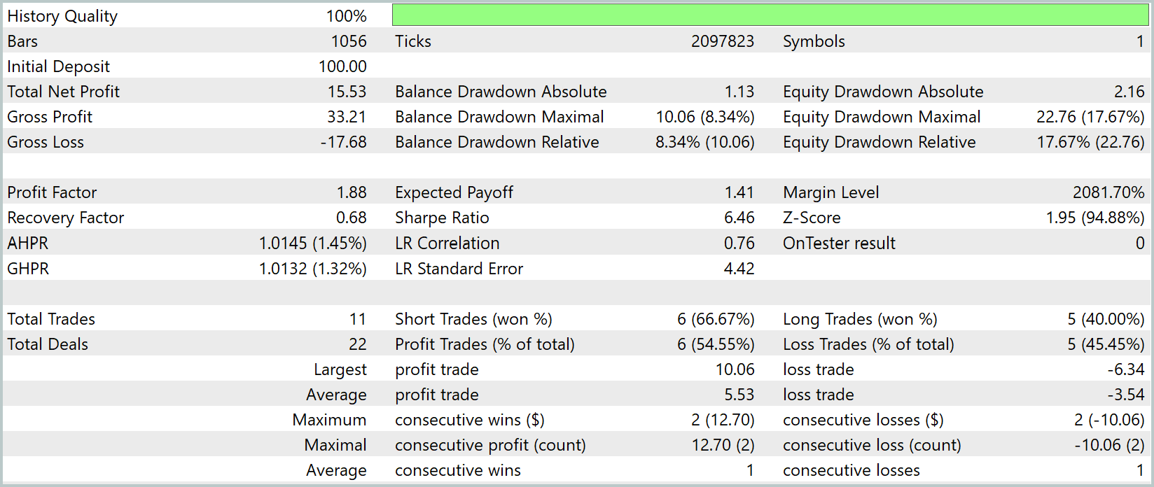
The final test was conducted using data from July–August 2025 — data that was entirely new and had not been used before. All parameters obtained in the previous stages were loaded without modification, ensuring an unbiased assessment of the model’s ability to generalize and of its robustness to new market conditions. The test results are presented below, demonstrating the effectiveness of a step-by-step approach to training the model and adapting it to real-world financial market conditions.

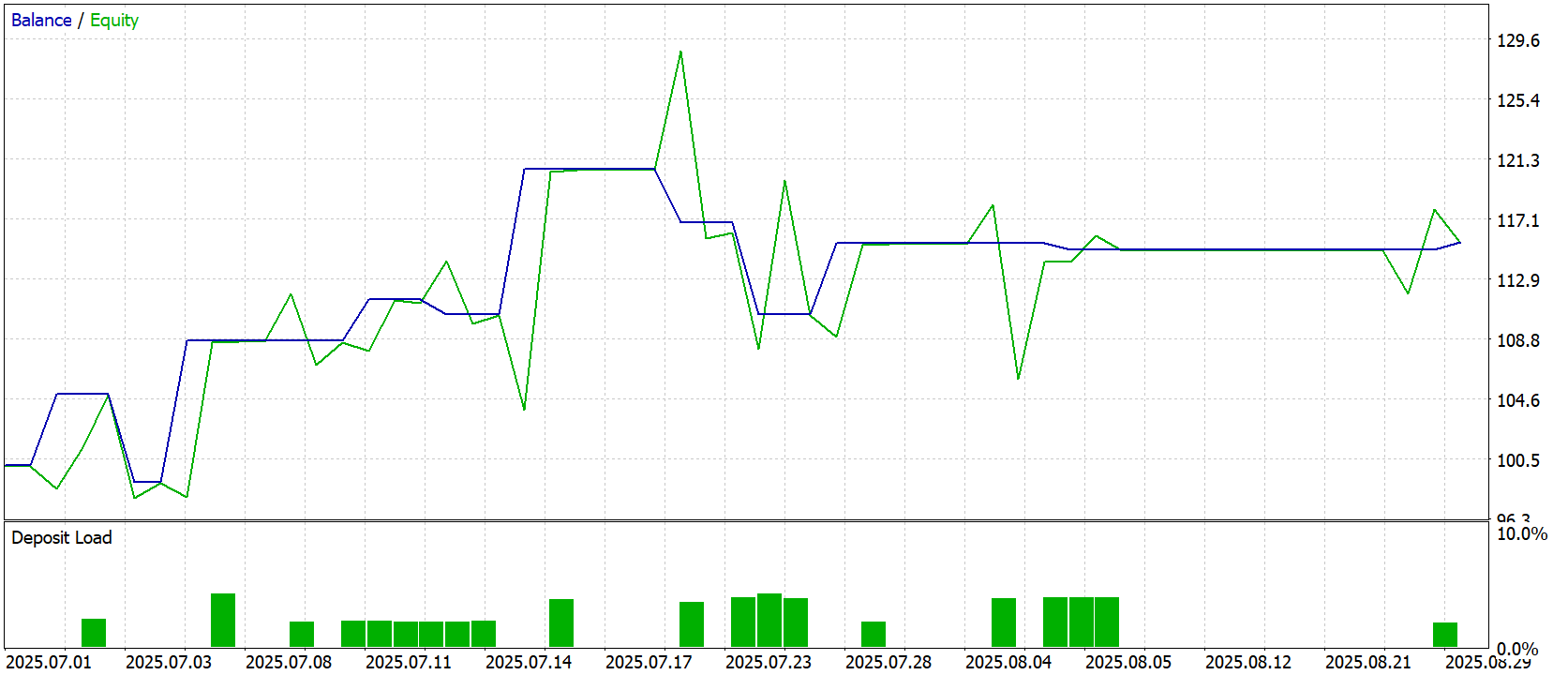
The test results demonstrate the model's effectiveness on previously unused data. The balance and equity chart shows a smooth, controlled increase in capital. At the same time, the balance shows a relatively stable trajectory, while equity reflects the short-term fluctuations typical of a real market environment. Occasional spikes and corrections can be observed, indicating the model's ability to adapt to unexpected market events while maintaining an overall positive trend.

The statistical metrics support the visual impression. The total profit was 15.53 USD on an initial deposit of 100 USD, corresponding to a moderate return with controlled risk. The maximum equity drawdown reached 22.76% — a relatively significant figure, but within the acceptable risk level for a test strategy. The profit factor (Profit Factor) is 1.88, confirming that profitable trades outnumber losing ones.

The model executed only 11 trading operations (22 trades), of which 54.55% were profitable. The average profit per trade was USD 5.53, and the average loss was USD 3.54, demonstrating a reasonable reward-to-risk ratio. The longest winning streak consisted of 2 trades totaling USD 12.70, and the longest losing streak consisted of 2 trades totaling USD -10.06. These metrics confirm that the model is capable of maintaining a balance between aggressiveness and stability without exposing capital to excessive risk.

Overall, the test results show that the model successfully integrates SpikingBrain approaches, is capable of processing dynamic financial signals, and can make controlled decisions in real-market conditions while maintaining stability and controlled returns.

Conclusion

The evolution of neural network architectures toward spiking models is opening up new horizons for trading. While transformers have proven their effectiveness in analyzing large volumes of market data and generating stable signals, spiking neurons bring us closer to systems that are more biologically plausible and energy-efficient. Their ability to handle temporal patterns and noisy data streams makes them promising for high-frequency trading and adaptive strategies.

However, the key challenge remains the same: integrating these models into real-world trading systems requires rigorous testing, risk assessment, and an understanding of the limitations of each architecture.

References

• SpikingBrain Technical Report: Spiking Brain-inspired Large Models
• Other articles in this series

Software used in this article

#	Name	Type	Description
1	Study.mq5	Expert Advisor	Expert Advisor for Offline Model Training
2	StudyOnline.mq5	Expert Advisor	Online Model Training Expert Advisor
3	Test.mq5	Expert Advisor	Model Testing Expert Advisor
4	Trajectory.mqh	Class Library	Structure for Describing the System State and Model Architecture
5	NeuroNet.mqh	Class Library	A class library for building a neural network
6	NeuroNet.cl	Library	Code Library for an OpenCL Program