

Regime Discovery by Structure: Implementing Toeplitz Inverse Covariance Clustering (TICC)
 909
 0

Introduction
Multi-symbol trading leads quickly to a covariance matrix, and that matrix fails twice. Estimated from a short window it is badly conditioned, so inversion is unstable. Separately, a correlation heatmap mixes direct and indirect links: a high value between two symbols cannot tell a direct link from a reflection of a third symbol they both follow. The inverse of the covariance matrix, the precision matrix, asks whether two symbols are still related once the rest of the basket is accounted for. For FX majors, that largely conditions away the shared dollar leg, at least its linear part.
We estimate it under an L1 penalty, so absent links become exact zeros, and we estimate it separately for each regime. The method is Toeplitz Inverse Covariance Clustering (TICC), by Hallac, Vare, Boyd and Leskovec, where a regime is not a level of volatility, but a dependency structure: which symbol's earlier bars are linked to which symbol's later bars, and at which lag. Everything here is native MQL5, with bundled ALGLIB only for the initial clustering.
We will cover:
- Precision Matrices and Partial Correlation
- Stacked Observations and the Block-Toeplitz Constraint
- The Toeplitz Graphical Lasso by ADMM
- Testing the Solver Before Trusting It
- From a Solver to Regimes
- Aligning and Scaling Real Data
- Choosing K, Lambda and Beta
- Putting It on a Chart Without Repainting
- What the Regimes Are, and What They Are Not
- Conclusion
Precision Matrices and Partial Correlation
Take five FX majors: EURUSD, GBPUSD, USDJPY, AUDUSD and USDCHF. Their correlation matrix holds large numbers almost everywhere and almost no information, because four of the five quote the same currency on one side. The narrower question is whether EURUSD still tells us anything about USDCHF once we know what the other three did on this bar. That is conditional dependence, and the precision matrix answers it.
Write the covariance matrix of the returns as S and its inverse as theta. The off-diagonal entries of theta convert into partial correlations:
p_ij = -theta_ij / sqrt( theta_ii * theta_jj )
That is the correlation between i and j with every other symbol's linear influence removed: scale free, and exactly zero under conditional independence. Those zeros are the point, and they are also the fragility: sampling noise leaves a directly inverted covariance with small non-zero numbers everywhere. The graphical lasso fixes it with an L1 penalty on the off-diagonal entries, so an absent edge claims conditional independence rather than weak correlation.

Fig. 1. The same five symbols under correlation and under partial correlation. Conditioning strips out most of the shared dollar leg and leaves a sparse graph.
Conditioning is linear. A common factor such as the dollar is shrunk, not deleted: with four other USD pairs in the basket it is pinned down well, so what remains of it is small, but nonlinear co-movement and anything driven from outside the basket stay in the estimate.
All of that concerns a single instant. What separates one regime from another is largely which symbol moves first, which needs a change of representation.
Stacked Observations and the Block-Toeplitz Constraint
To let a precision matrix express lead and lag, a bar stops being a vector of n returns and becomes n returns over the last w bars, flattened into one vector: the stacked observation, which every stage of the pipeline works on.
X_t = [ r_{t-w+1} ; ... ; r_{t-1} ; r_t ] With n symbols over w bars, X_t has length nw. Entry (i*n + j) holds series j at lag block i, counting from the oldest bar. A regime is modelled as a Gaussian over this vector, so theta is nw by nw, 25 by 25 here. The payoff is the block structure. Read theta as a w by w grid of n by n blocks: the diagonal block holds the contemporaneous graph of section one, and each step off it adds one more bar of separation. That layout contract sits at the top of TICC_Types.mqh.

Fig. 2. Five symbols over five bars stack into one vector of length 25, and the 25 by 25 precision matrix partitions into blocks by lag distance.
Why theta is block-Toeplitz. A regime is the same regime at every bar inside it, which makes the covariance of the stacked vector exactly block-Toeplitz: the block linking lag block i to lag block j depends only on j - i. Its inverse is not exactly block-Toeplitz; even for a single AR(1) series, the first and last diagonal entries of the inverse differ from the interior ones. TICC imposes the structure on theta anyway, as a modelling assumption rather than a consequence of stationarity, and what it buys is economy. Without it the model carries w times more free parameters than the data supports and learns that "the third bar behaves differently from the fourth", an artefact of where the window fell. This is what separates TICC from clustering feature vectors with k-means.
Turning the constraint into a lookup
Rather than solve unconstrained and project afterwards, we map every entry in advance to the group of entries it must equal, so the constraint becomes how the matrix is addressed. With p and q the position inside a lag block and d the block distance, the canonical key is:
d > 0   ->  ( d, p, q)
d < 0   ->  (-d, q, p)
d = 0   ->  ( 0, min(p,q), max(p,q))
The transpose in the middle line and the min and max in the diagonal block send (r,c) and (c,r) to the same key, so a matrix built from group values is symmetric by construction, not by correction. CTiccGroups in TICC_Math.mqh owns the map:
   for(int r = 0; r < m_dim; r++)
     {
      for(int c = 0; c < m_dim; c++)
        {
         int bi = r / n, p = r % n;
         int bj = c / n, q = c % n;
         int d  = bj - bi;

         int ad = (d >= 0 ? d : -d);
         int kp = p, kq = q;

         //--- transpose below the diagonal, and inside the d = 0 block,
         //--- so that (r,c) and (c,r) always land on the same key.
         if(d < 0 || (d == 0 && p > q))
           {
            kp = q;
            kq = p;
           }

         int raw = ad * n * n + kp * n + kq;
         if(intern[raw] < 0)
           {
            intern[raw] = m_count;
            ArrayResize(m_size, m_count + 1);
            ArrayResize(m_lag,  m_count + 1);
            ArrayResize(m_diag, m_count + 1);
            m_size[m_count] = 0;
            m_lag[m_count]  = ad;
            m_diag[m_count] = (ad == 0 && kp == kq);
            m_count++;
           }

         int g = intern[raw];
         m_id[r * m_dim + c] = g;
         m_size[g]++;
        }
     }
Interning a key the first time it is seen keeps indices dense and stably ordered, and each group records its lag distance and whether it is a variance term, both of which the penalty needs. Here the 625 entries of theta resolve to 115 groups, the real free parameters of each regime's precision matrix. Counting non-zero entries instead overstates complexity more than fivefold and picks the wrong number of regimes.
Of those 115 groups, five are the variances on the diagonal, twenty link a symbol to its own earlier bars, and ninety link different symbols. The full model adds a mean per regime, the switching penalty and the selection choices on top, so 115 is the size of one regime's graph, not the dimension of everything that is fitted.
The Toeplitz Graphical Lasso by ADMM
What remains is estimating theta from data. For one regime the problem is:
min  -log|theta| + trace(S theta) + || Lambda o theta ||_1
over theta positive definite and block-Toeplitz
S is the empirical covariance of that regime's stacked observations, o the elementwise product, Lambda the per-entry penalty weights. The first two terms are the Gaussian negative log-likelihood; the third drives entries to zero. S also carries a small ridge, 1e-4 by default, which keeps the first eigendecomposition finite when a regime is thinly populated.
Nothing minimises that directly: the log-determinant is smooth and wants density, the L1 term is non-smooth, and block-Toeplitz is a hard constraint. ADMM splits it across two variables forced to agree. Theta takes the log-determinant and trace, a second matrix Z takes the L1 penalty and the Toeplitz structure, theta = Z ties them, and a scaled dual U tracks their disagreement.
The theta step has a closed form
Minimising over theta means solving:
min -log|theta| + trace(S theta) + (rho/2) || theta - Z + U ||_F^2
Setting the gradient to zero gives the optimality condition:
rho*theta - theta^-1 = rho*(Z - U) - S = M This looks like it needs a matrix inversion inside an iteration, but theta and M commute at the optimum, so they share an eigenbasis. Writing M = Q diag(e) Q^T and theta = Q diag(x) Q^T decouples the matrix equation into nw scalar equations:
rho*x - 1/x = e That is a quadratic in x, and taking the positive root gives:
x_i = ( e_i + sqrt( e_i^2 + 4 rho ) ) / (2 rho)
Because rho is positive the square root always exceeds the absolute value of e_i, so x_i is strictly positive for every eigenvalue, whatever S looked like. Theta is positive definite by construction, S is never inverted, and the whole step costs one symmetric eigendecomposition per iteration.

Fig. 3. The theta update in the eigenbasis of M. Each eigenvalue solves the same scalar quadratic, whose positive root keeps theta positive definite.
The Z step is where the structure lives
The Z update carries both the L1 penalty and the block-Toeplitz constraint, which is where the group map pays off. Every entry in a group shares one value and one penalty weight, so the group's subproblem collapses to a scalar minimisation, and averaging then thresholding is its exact proximal operator rather than a projection bolted on afterwards.
//+------------------------------------------------------------------+
//| Z step: average each Toeplitz group, then soft-threshold it.     |
//|                                                                  |
//|  Averaging first is not a heuristic. Minimising the group's own  |
//|  objective over a single shared value leaves the mean as the     |
//|  only term the quadratic sees, so the scalar problem reduces to  |
//|  a lasso about that mean and the threshold is lambda/rho.        |
//+------------------------------------------------------------------+
void CGraphicalLasso::UpdateZ(const matrix &a, const double rho, int &nnz)
  {
   int ng = m_groups.Count();
   ArrayInitialize(m_gsum, 0.0);

   for(int r = 0; r < m_dim; r++)
      for(int c = 0; c < m_dim; c++)
         m_gsum[m_groups.Id(r, c)] += a[r][c];

   nnz = 0;
   for(int g = 0; g < ng; g++)
     {
      double mean = m_gsum[g] / (double)m_groups.Size(g);
      m_gval[g] = TiccSoftThreshold(mean, m_lam[g] / rho);
      if(m_gval[g] != 0.0)
         nnz++;
     }

   for(int r = 0; r < m_dim; r++)
      for(int c = 0; c < m_dim; c++)
         m_Z[r][c] = m_gval[m_groups.Id(r, c)];
  }
Three passes: gather each group's sum, threshold its mean, scatter it back. Since every entry is written from its group's single value, the result is exactly symmetric and block-Toeplitz to machine precision.
Penalty weights and the lag taper
BuildPenalty makes two deliberate choices. Diagonal variance terms are never penalised, since shrinking them biases the log-determinant for reasons unrelated to dependency structure. And the weight grows with lag distance:
lambda_d = lambda * exp( d^2 / (2 sigma^2) )
A link at four bars of separation therefore clears a stiffer threshold than a contemporaneous one, encoding the prior that distant lags are sparser. The value used is 2.5; setting taper_sigma to zero gives a flat penalty, and section nine reports what that costs.
The full iteration
Both steps sit inside one loop. This excerpt picks it up at the Z step, where the dual ascent, the stopping test and the rho adaptation live:
      //--- Z step, then the dual ascent.
      matrix z_old = m_Z;
      matrix a     = theta + m_U;
      UpdateZ(a, rho, nnz);
      m_U = m_U + theta - m_Z;

      //--- Boyd's stopping rule, absolute plus relative.
      double r_pri = (theta - m_Z).Norm(MATRIX_NORM_FROBENIUS);
      double r_dua = rho * (m_Z - z_old).Norm(MATRIX_NORM_FROBENIUS);

      double n_th = theta.Norm(MATRIX_NORM_FROBENIUS);
      double n_z  = m_Z.Norm(MATRIX_NORM_FROBENIUS);
      double n_u  = m_U.Norm(MATRIX_NORM_FROBENIUS);

      double eps_pri = scale * cfg.admm_tol_abs
                       + cfg.admm_tol_rel * MathMax(n_th, n_z);
      double eps_dua = scale * cfg.admm_tol_abs
                       + cfg.admm_tol_rel * rho * n_u;

      rep.iterations = it;
      rep.r_primal   = r_pri;
      rep.r_dual     = r_dua;

      if(r_pri <= eps_pri && r_dua <= eps_dua)
        {
         rep.converged = true;
         break;
        }

      //--- the two tests are mutually exclusive, so they need no else.
      if(cfg.adapt_rho && r_pri > 10.0 * r_dua)
        {
         rho *= 2.0;
         m_U /= 2.0;
        }
      if(cfg.adapt_rho && r_dua > 10.0 * r_pri)
        {
         rho /= 2.0;
         m_U *= 2.0;
        }
     }
Stopping follows Boyd's rule on the primal residual, how far theta and Z have drifted apart, and the dual, how much Z moved. The scale factor on the absolute tolerance is the square root of the entry count, so a fixed tolerance keeps its meaning as the problem grows; rho is rebalanced when the residuals diverge tenfold.
On exit the solver exposes two matrices agreeing to the primal tolerance but not identical: theta, positive definite and used for likelihoods, and Z, carrying the exact zeros and block-Toeplitz structure a graph is drawn from.
Testing the Solver Before Trusting It
A graphical lasso that has silently failed to converge still returns a plausible-looking matrix: labels appear, the indicator paints, nothing complains. The only defence is data whose answer is already known. Such checks confirm specific properties on cases with a known answer; they do not prove the solver correct on every input, but a solver that fails them is certainly wrong.
TICC_SolverTest.mq5 runs six groups of checks in order of dependency, so the first failure names the lowest broken layer rather than a symptom. It works at n = 3 over w = 3, small enough to check by eye, and the group count is verified against a formula derived independently of the code: n(n+1)/2 at lag zero plus n^2 per remaining lag. The first line pins a convention nothing else would catch, since the theta update assumes eigenvectors arrive in the columns of Q.
[PASS] eigenvectors are in columns            col err 2.109e-15 vs row err 2.835e+00
[PASS] group count matches the shape          n=3 w=3 gave 24, expected 24
[PASS] group count matches the shape          n=5 w=5 gave 115, expected 115
[PASS] rebuilt matrix is symmetric            max asymmetry 0.0e+00
[PASS] rebuilt matrix is block-Toeplitz       max block drift 0.0e+00
[PASS] group sizes tile the matrix            625 entries covered, matrix holds 625
The substantive test builds a precision matrix with a known sparsity pattern, draws samples from the corresponding Gaussian, and asks the solver to recover the planted edges:
[PASS] samples reproduce the covariance       relative max error 0.0092 over 6000 draws
[PASS] solver converges                       19 iterations, primal 1.82e-04, dual 2.65e-05, rho 1.000
[PASS] solution is positive definite          min eigenvalue 0.4821, log|theta| = -0.9025
[PASS] all true edges recovered               3 true, 3 found, 0 missed, 0 spurious
[PASS] large lambda empties the graph         0 edges left, 3 variance terms
[PASS] zero lambda gives the Toeplitz MLE     relative gap to inv(S) 0.0072
The positive-definiteness check factorises theta and reports its smallest eigenvalue, the direct evidence. Compute such a value before the call that reports it: MQL5 does not evaluate arguments left to right, so a message formatted in the same call can read the variable before the function that fills it has run.
The last two lines are the limiting behaviours. At a large lambda only the three diagonal variance terms survive, since they are never penalised, so the graph has no edges while theta remains a valid diagonal precision matrix. At lambda = 0 the solver returns the block-Toeplitz constrained maximum-likelihood estimate, not inv(S). The two are close here, a residual of 0.0072, only because the synthetic S was drawn from a block-Toeplitz truth; a covariance with no such structure would leave a larger gap.
A platform behaviour that will break your solver
The native symmetric eigendecomposition rejects a matrix that is asymmetric in the last bit. A covariance built as X^T X returns entries (i,j) and (j,i) differing by around 1e-17, since the dot products accumulate in different orders. EigenSymmetricDC refuses such a matrix outright. Hand-built test matrices are assigned in pairs and pass perfectly, so this shows up only on real data. Symmetrise before every call:
//+------------------------------------------------------------------+
//| Symmetric eigendecomposition: M = Q * diag(d) * Q^T.             |
//|                                                                  |
//|  Eigenvectors come back in the COLUMNS of Q, matching the numpy  |
//|  convention the MQL5 matrix methods follow. TICC_SolverTest      |
//|  reconstructs M from the factors and fails loudly if that ever   |
//|  stops being true, because every downstream sign would flip      |
//|  silently otherwise.                                             |
//|                                                                  |
//|  The input is symmetrised first, and that is not defensive       |
//|  padding. A covariance built as X^T X comes back from the BLAS   |
//|  with entry (i,j) and entry (j,i) differing in the last bit or   |
//|  two, because the two dot products are accumulated in different  |
//|  orders. EigenSymmetricDC rejects such a matrix outright rather  |
//|  than tolerating the drift, so a solver that skips this step     |
//|  fails on real data while passing every hand-built test.         |
//+------------------------------------------------------------------+
bool TiccSymEig(const matrix &m, matrix &q, vector &d)
  {
   matrix work = (m + m.Transpose()) * 0.5;
   if(work.EigenSymmetricDC(EIGVALUES_V, d, q))
      return(true);

//--- fall back to the general solver; on a symmetric input it agrees.
   work = (m + m.Transpose()) * 0.5;
   return(work.Eig(q, d));
  }
From a Solver to Regimes
The solver estimates one regime. A clustering alternates two steps until the labels stop moving: given an assignment, fit each regime's precision matrix; given those matrices, relabel every observation. The relabelling is the second idea that makes TICC what it is.
Why a bar is not sent to its nearest regime
Assigning each observation independently to whichever regime explains it best produces labels that flip on single-bar noise, which no trader can act on and which contradicts the premise: if regimes were not persistent, block-Toeplitz would be meaningless.
Instead the whole label path is chosen at once, minimising:
sum_t -log p( X_t | regime_t ) + beta * switches
Beta buys temporal coherence in units of log-likelihood: a switch must explain the data at least beta better than staying put. Dynamic programming solves this exactly, with the Viterbi recursion an HMM uses, hence AssignViterbi; what differs is the state, a sparse precision matrix over a stacked observation rather than a mean and a variance. Beta is in nats against a 25-dimensional Gaussian, so it does not transfer between problems. Tune it by the regime durations it produces.
A naive recursion is O(K^2) per bar, since each state considers every predecessor. Here the switching cost does not depend on which regime is left, only that one is, so the best predecessor for state c is either c itself or the globally cheapest state plus beta, which makes the step O(K).
   for(int t = 1; t < m_nobs; t++)
     {
      int    best_prev = 0;
      double best_val  = j_prev[0];
      for(int c = 1; c < k; c++)
        {
         if(j_prev[c] < best_val)
           {
            best_val  = j_prev[c];
            best_prev = c;
           }
        }

      for(int c = 0; c < k; c++)
        {
         double stay = j_prev[c];
         double swap = best_val + m_cfg.beta;
         if(stay <= swap)
           {
            j_cur[c]      = all_cost[t * k + c] + stay;
            bp[t * k + c] = c;
           }
         else
           {
            j_cur[c]      = all_cost[t * k + c] + swap;
            bp[t * k + c] = best_prev;
           }
        }
      for(int c = 0; c < k; c++)
         j_prev[c] = j_cur[c];
     }
Per-regime costs are evaluated once into all_cost and reused, since a Mahalanobis product inside that loop would dominate the entire algorithm's run time.
Seeding, and keeping regimes viable
The starting assignment comes from bundled ALGLIB k-means, which only has to land in the right basin; the dynamic programming step supplies the temporal structure it cannot see. A regime below the viability floor of twenty observations is refilled from the points furthest from the largest regime's centre, since a handful of members gives a covariance singular in every unobserved direction.
A stopping rule that must not be the iteration cap
Stopping when no observation changes label is essentially impossible to meet on several thousand observations: a handful of bars oscillate on a decision boundary while the model behind them is stable, so the iteration cap ends every run and becomes a hidden hyperparameter. Two changes remove the problem:
//--- Stopping only at zero moved labels is unmeetable here, which lets
//--- em_max_iter silently decide the answer. A tolerance ends the loop
//--- on the model settling, and the best iterate is kept because the
//--- assignment step is not monotone in likelihood.
   double ll        = 0.0;
   double best_ll   = 0.0;
   bool   have_best = false;
   int    best_labels[];
   int    tol = MathMax(1, m_nobs / 500);

   for(int it = 1; it <= cfg.em_max_iter; it++)
     {
      if(!RefitClusters())
         return(false);

      int fresh[];
      ll = AssignViterbi(fresh);

      if(!have_best || ll > best_ll)
        {
         best_ll = ll;
         ArrayCopy(best_labels, fresh);
         have_best = true;
        }

      int moved = 0;
      for(int i = 0; i < m_nobs; i++)
         if(fresh[i] != m_label[i])
            moved++;

      ArrayCopy(m_label, fresh);
      ReseedSmall();

      rep.em_iterations = it;
      if(moved <= tol)
        {
         rep.converged = true;
         break;
        }
     }
The first is a tolerance: stop when fewer than one observation in five hundred changes label. The second matters more. The alternation is not monotone in likelihood. The assignment step minimises the path cost above, likelihood plus the switching penalty, while the best iterate is scored on the Gaussian log-likelihood alone, beta excluded, and refilling an undersized regime moves points by rule rather than by either objective. The final iterate is therefore not reliably the best; keeping the best-scoring one makes the fit reproducible wherever the cap falls. Without both, no configuration converges; with them, five of six converge in six to eight iterations.
Aligning and Scaling Real Data
Alignment is not optional
A precision matrix describes what happens at the same instant across several symbols. Assemble rows by bar index rather than timestamp and one missing bar shifts a symbol's column against the others, so every lag block after it describes a lead-lag relationship that never happened. Symbols go quiet at different minutes around the rollover, so this is routine. CTiccData keeps only timestamps present on every symbol and reports the drops; a large count means the basket or timeframe is a poor fit. Here it reports zero across 11,880 rows, but swap USDJPY for a CFD and that changes.
Scaling decides what the clustering can see
This choice shapes the result more than any other. Standardising over the whole sample divides a violent week and a quiet one by the same number, so clustering gets volatility level as a feature and returns a volatility detector disguised as a dependency model. A causal rolling standardisation divides each return by a sigma from the bars strictly before it, so the slow-moving volatility level goes and the shape of the co-movement survives. It does not remove everything: a bar that surprises its own trailing sigma still stands out, and the standardised returns keep their fat tails.
   matrix out = matrix::Zeros(m_rows - win, m_n);

   for(int s = 0; s < m_n; s++)
     {
      double sum = 0.0, sumsq = 0.0;
      for(int t = 0; t < win; t++)
        {
         double v = m_returns[t][s];
         sum   += v;
         sumsq += v * v;
        }

      for(int t = win; t < m_rows; t++)
        {
         double mu  = sum / win;
         double var = sumsq / win - mu * mu;
         double sd  = (var > 0.0 ? MathSqrt(var) : 0.0);
         if(sd <= 0.0)
           {
            PrintFormat("TICC data: %s is flat inside the rolling window",
                        m_symbols[s]);
            return(false);
           }
         out[t - win][s] = (m_returns[t][s] - mu) / sd;

         double drop = m_returns[t - win][s];
         double add  = m_returns[t][s];
         sum   += add - drop;
         sumsq += add * add - drop * drop;
        }
Choosing K, Lambda and Beta
Three parameters shape the result: K, the L1 weight lambda, and the switching penalty beta. TICC_Fit.mq5 runs the pipeline and splits it into a training block and a causally labelled held-out block. The fit never sees the held-out block, but the choice of K and beta below does, so it serves as a validation block rather than an untouched final test.
Every number below uses the same inputs: the five majors in that column order, H1, 12,000 bars, InpWindow 5, InpLambda 0.01, InpTaper 2.5, InpTrainFrac 0.67, InpCommitLag 5, InpEmIters 60, InpVolWindow 120, with InpForceK pinned 3 to 6 and InpBeta 60 or 100. That leaves 11,880 return rows, split 7,959 and 3,921. Each block is stacked separately, so the fit works on 7,955 stacked observations and the held-out block supplies 3,917.
Do not select on BIC here
BIC is the natural first choice and here it misleads. Its penalty counts non-zero groups as free parameters, which is the right count for an unpenalised maximum-likelihood fit but not for a lasso estimate whose surviving entries are shrunk, and its likelihood is scored on the very label path the fit chose. Under those conditions crushing the graph reads as an improvement: at lambda = 0.10 the dominant regime kept 13 groups out of 115, and BIC picks that model confidently. On held-out data it scores 0.38 nats per bar against a single-Gaussian null, against 2.7 for the best model below.
What replaces it is held-out log-likelihood against a single-Gaussian null fitted on the same training block, which NullLogLik computes. It works as a gate: a model that does not clearly beat the null is rejected, and among the models that pass, the choice is made on regime duration and occupancy. The script still prints BIC's pick, so you can watch it choose confidently and badly.
The selection study
Sweeping K and beta on converged fits gives:
| K | beta | converged | held-out gain (nats/bar) | structure spread | median duration (bars) | held-out occupancy (%) |
|---|---|---|---|---|---|---|
| 5 | 60 | yes (8) | 2.73 | 3.75x | 9 | 47.0 / 41.8 / 7.1 |
| 5 | 100 | yes (8) | 1.37 | 3.86x | 20 | 86.5 dominant |
| 4 | 60 | yes (8) | 2.32 | 3.64x | 15 | 82.7 dominant |
| 4 | 100 | no (60) | 1.17 | 4.33x | 26 | 91.7 dominant |
| 6 | 100 | yes (8) | 1.85 | 3.71x | 17 | 68.5 / 15.3 / 13.0 |
| 3 | 100 | yes (6) | 2.03 | 1.72x | 18 | 78.1 / 16.4 / 5.4 |
"Converged" carries the EM iteration count, so "no (60)" ran to the cap. "Structure spread" is the ratio between the most and least tightly coupled regime by mean absolute partial correlation, and "held-out occupancy" lists the three largest regimes, making a degenerate fit visible at a glance.
Raising beta lengthens regimes, but past a point occupancy concentrates until one regime holds almost every bar. We take forward K = 6, lambda = 0.01, beta = 100. It does not have the best likelihood; it is the only row that passes every rule in the "When to stop" list at the end of section nine: held-out gain clearly positive, structure spread above 2x, median duration at least three times the 5-bar commit lag, and no regime above about 70% of held-out bars. K = 5, beta = 60 scores better, but its 9-bar median loses half the regime before the label lands. K = 5, beta = 100 and K = 4, beta = 60 put over 80% of bars in one regime, K = 4, beta = 100 did not converge, and K = 3 fails on spread. The binding constraint on a chart is duration against commit lag: a 17-bar median against a 5-bar lag leaves about 70 percent of the regime ahead when the label lands.
Putting It on a Chart Without Repainting
Everything so far is a batch algorithm: the dynamic programming step runs a backward pass over the whole sequence, so every label was computed with knowledge of the future. Plot those and the indicator repaints, and is worthless.
Fit once, assign forever
Fitting costs minutes; labelling a bar costs microseconds. A model file separates them: SaveModel writes the regimes, the indicator only loads and assigns. It also records symbol names in column order plus the standardisation mode and window, without which the same symbols in a different order would score against the wrong quantity.
Committing a label so it can never move
The causal counterpart freezes the regimes and runs the same recursion forward only. A label is committed a fixed number of bars after its own bar, and is never revised afterwards:
         int head = 0;
         for(int c = 1; c < k; c++)
            if(j_prev[c] < j_prev[head])
               head = c;

         int node = head;
         for(int s = t; s > t - lag; s--)
            node = bp[s * k + node];
         labels[t - lag] = node;
At each bar the recursion walks back exactly lag steps from the current best state and commits the label it lands on. Later bars could in principle still have changed the optimal path that far back; the label is frozen by design, not because its uncertainty has gone, and that freezing is what makes the indicator non-repainting. A longer lag makes such a revision less likely, at the price of a later label. The most recent bars are genuinely undecided, so the rendering shows nothing there, and everything reported out of sample comes from this routine.
Two platform behaviours that will make an indicator look broken
The first concerns cross-symbol history. An indicator drawing on one symbol needs bars from four others, routinely still downloading at the first tick, so a first pass that paints nothing is normal. The trap is the recalculation guard, which skips the work when the bar count has not moved:
//--- latched only after a pass that painted, so a basket symbol whose
//--- history has not arrived yet cannot latch the guard forever.
   if(prev_calculated > 0 && rates_total == g_last_bars)
      return(rates_total);
The guard itself is correct. What matters is where the value it tests against gets written:
   int painted = g_live.Update(_Period, slice, want, InpCommitLag,
                               labels, margins);
   if(painted <= 0)
     {
      static int complained = 0;
      if(complained < 3)
        {
         PrintFormat("TICC regime: nothing labelled over %d bars yet,"
                     " will retry on the next tick", want);
         complained++;
        }
      //--- zero, not rates_total: a non-zero BarsCalculated would let
      //--- every iCustom caller read an empty buffer as a final answer.
      ShowStatus(TICC_LABEL_NONE, 0.0);
      return(0);
     }

   g_last_bars = rates_total;
Note where g_last_bars is assigned. Latching the bar count before the work turns one early failure into a permanent one: every later tick matches the guard and never retries, so the window stays empty until a new bar forms. Latch only after a pass that painted.
The second concerns readiness. Returning rates_total when nothing was painted makes BarsCalculated non-zero, so every iCustom caller reads an empty buffer as a finished answer.
Reading the output
The indicator renders as a flat coloured ribbon, ordered cool to hot by how tightly each regime couples the basket. Regime indices are arbitrary and unstable across refits, so ordering by coupling is what makes a colour mean the same thing every time.
The ribbon says which regime; the panel says what it is, drawing the precision matrix as a graph: nodes are symbols, chords are contemporaneous partial correlations, arrows run from the earlier bar to the later one at one bar of separation, and a ring is a symbol's own one-bar term. An arrow is a lagged conditional dependence, a matter of time order rather than causation: once the rest of the basket is known, the earlier move of one symbol carries information about the later move of another, which is not the same as one driving the other. TICC_GraphPanel.mq5 loads the model itself rather than reading the ribbon through iCustom, so it works alone, but its InpCommitLag must match.
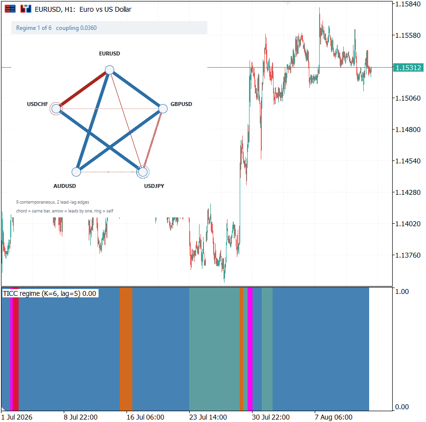
Fig. 4. The regime ribbon and the dependency graph of the active regime. The rightmost bars are intentionally unpainted: that is the commit lag.
The graph doubles as a check on the pipeline. EURUSD and USDCHF come out joined by a thick negative chord, while EURUSD and GBPUSD, and AUDUSD and GBPUSD, come out positive: correct FX behaviour falling out of the estimated precision matrix.
Running it end to end
- Run TICC_SolverTest.mq5 on any chart. It needs no market data and should print twenty passing checks.
- Run TICC_Fit.mq5 with the inputs from section seven and InpSaveModel set to a file name, every basket symbol in Market Watch first. It writes the model to MQL5\Files\TICC\ and checks the reloaded copy reproduces the same labels.
- Attach TICC_Regime.mq5 to any chart with InpModelFile set to that file. The model carries its own basket, so the chart symbol need not be in it.
- Attach TICC_GraphPanel.mq5 to the same chart, same model file, same commit lag.
What the Regimes Are, and What They Are Not
The regimes might be volatility states with extra steps. Section six divides the local volatility level out, so any difference that survives is either structure or volatility surprise, and the fit measures both.
The regimes are not only volatility states
The fit reports volatility spread, the ratio of the noisiest regime to the quietest by root mean square of the standardised returns, and structure spread, the same ratio on mean absolute partial correlation and therefore scale free. A seeded run gives 4.88x volatility and 3.87x structure, and the structure figure holds at 3.6x to 4.3x for every K of four or more, falling to 1.72x only at K = 3. A value near one would have settled the question against the method.
The volatility figure looks like the opposite conclusion, but these returns are already divided by a sigma from the previous 120 bars, so 4.88x measures surprise against what the recent past predicted, not volatility level. Only the structural figure is scale free, which is why the argument rests on it. The regimes do differ in surprise as well, so they are not purely structural; the claim is only that structure differs too, by a measure that volatility cannot move. Five of the six regimes are listed below; the sixth holds 2.5% of training bars.
| regime | share of training bars | non-zero groups | mean abs partial corr |
|---|---|---|---|
| calm (dominant) | 49.0% | 28 | 0.036 |
| transitional | 22.3% | 44 | 0.043 |
| transitional | 25.5% | 51 | 0.036 |
| rare | 0.4% | 97 | 0.124 |
| rare | 0.3% | 95 | 0.133 |
Non-zero groups count every surviving group, including the five variances that are never penalised, and mean absolute partial correlation averages every off-diagonal pair of the 25 by 25 matrix, zeros included. The dominant regime is close to conditionally independent: 28 groups out of 115, so 23 dependencies, at 0.036 mean partial correlation. Once most of the dollar leg is conditioned away the majors have little left to say to each other, while the two rare regimes carry nearly a hundred groups and three to four times the coupling. Read as stress, that would be diversification failing when it is needed; the small-sample control below shows how little of it survives once regime size is accounted for.
Does it replicate?
Since k-means seeds the alternation, refitting from another seed asks whether the regimes belong to the data or to where the search began. Occupancy moves a long way, the 49.0% regime splitting into 43.6%, 34.0% and 19.0%, but the populated regimes stay sparse, 23 to 42 groups at 0.036 to 0.039, regimes under one percent again carry 96 to 107, and held-out gain is 2.27 nats per bar. Other seeds can land far from both fits, as the note in section seven shows, so a single fit is one draw from a seed-dependent set.
How much of it is sample size?
The rare regimes hold a few dozen windows each, and a graph estimated from so few is dense whatever the market was doing. TICC_Fit.mq5 measures this directly: it draws as many windows as the smallest regime holds, at random, from the largest regime, fits them exactly as a regime is fitted, and repeats that InpControlDraws times, 20 by default. A calm sample of the same size shows what size alone produces.
On a refit of the same window, where the two rare regimes held 22 and 38 windows, twenty draws of 22 calm windows came out with 87 to 100 groups, 92 on average, against 102 for the rare regime and 43 for the full calm regime it was drawn from. The density is sample size. The coupling is partly not: the draws averaged 0.089 mean absolute partial correlation against 0.120 and 0.127 for the rare regimes, about 1.4 times more. Those regimes' bars are also three to seven times more volatile than the calm ones, and correlations measured on volatile bars are biased upward (Forbes and Rigobon, 2002), so even that residual is an upper bound.
What the two preprocessing choices bought
Changing one at a time. Whole-sample standardisation, with its mean and sigma taken from the training block only so that nothing from the held-out block reaches the scaling, scores better on held-out likelihood: on the same window and seed, 2.73 nats per bar against 2.20 for the rolling version, but it puts 80.0% of held-out bars into a single regime against 41.0%. It bought its likelihood by describing one state well and saying almost nothing otherwise, so on likelihood alone the wrong variant wins. In the replication fit, turning the taper off raised surviving groups from 404 to 458 and changed nothing else, so it drops about one edge in eight, the long-lag ones it distrusts, at no cost.
What this does not do
- Regimes drift between the training and held-out blocks, and the direction is not stable. The dominant regime grew from 49.0% of training bars to 68.5% of held-out bars, while the seeded re-fit drifted the other way. Measure occupancy on your own split.
- Regime duration is short relative to the commit lag. The 17-bar median is usable but not comfortable, and it moves between windows: the verification run gave 15. Raising beta lengthens regimes but costs fit quality steeply.
- The rare regimes are rare. Two of the six hold around thirty stacked observations each, against 115 groups to estimate. Every regime is solved with the same lambda against its own average covariance, whatever its size, while the sampling noise in a correlation from thirty observations is around 0.18, far above lambda = 0.01, so almost every group survives the threshold. The control above confirms it: their density is what a sample that small produces, and only a modest excess of coupling remains. Do not read them as stress regimes.
When to stop
- Stop tuning lambda when the dominant regime holds roughly 20 to 40 non-zero groups. Far fewer means the graph has been crushed; far more means the penalty does no work.
- Stop tuning beta when the median regime duration is at least three times your commit lag and no regime exceeds about 70% of held-out bars. Both conditions, not either.
- Accept the model when held-out gain over the null is clearly positive and structure spread exceeds about 2x. Reject it if the solver did not converge or the EM loop hit its cap.
Conclusion
We set out to replace a correlation heatmap with a sparse dependency graph. What that took:
- The precision matrix is the object worth estimating. Partial correlation conditions away most of the dollar leg, linearly, and the L1 penalty turns what remains into exact zeros.
- Block-Toeplitz is what makes this more than clustering. Grouping entries up front makes symmetry structural, gives the Z step an exact proximal operator, and leaves each regime's precision matrix with 115 free parameters, not 625.
- The theta update needs no matrix inversion. One scalar quadratic per eigenvalue keeps theta positive definite however badly conditioned S was.
- Regimes must be chosen as a path, and because the switching penalty is uniform the recursion costs O(K) per bar.
- Calm markets are close to conditionally independent. The populated regimes keep a few dozen groups out of 115 across seeds. The rare regimes come out dense, but a calm sample of the same size is nearly as dense; what remains is about 1.4 times more coupling, at most.
- Gate on held-out likelihood, not BIC, which here rewards a penalty high enough to destroy the graph it is selecting; then choose among the models that pass on regime duration and occupancy.
This stops short of turning the precision matrix into position sizes. The estimate is well conditioned and positive definite, which is what a sizing rule needs, but choosing the rule is a different article. Possible extensions are a wider basket, a longer timeframe, and cross-asset baskets.
References
- Hallac, D., Vare, S., Boyd, S. and Leskovec, J. (2017). Toeplitz Inverse Covariance-Based Clustering of Multivariate Time Series Data. KDD 2017, 215-223.
- Boyd, S., Parikh, N., Chu, E., Peleato, B. and Eckstein, J. (2011). Distributed Optimization and Statistical Learning via the Alternating Direction Method of Multipliers. Foundations and Trends in Machine Learning 3(1), 1-122.
- Friedman, J., Hastie, T. and Tibshirani, R. (2008). Sparse Inverse Covariance Estimation with the Graphical Lasso. Biostatistics 9(3), 432-441.
- Dempster, A. P. (1972). Covariance Selection. Biometrics 28(1), 157-175.
- Forbes, K. J. and Rigobon, R. (2002). No Contagion, Only Interdependence: Measuring Stock Market Comovements. Journal of Finance 57(5), 2223-2261.
Getting the Source Code via MQL5 Algo Forge
All source files are attached to this article below, but the full repository is also available on MQL5 Algo Forge, the community's Git-based platform for sharing and collaborating on trading projects.
| File name | Description |
|---|---|
| MQL5\Include\TICC\TICC_Types.mqh | Configuration, regime and report structures, project file paths |
| MQL5\Include\TICC\TICC_Math.mqh | Group map, penalty taper, symmetric eigendecomposition, log-determinant |
| MQL5\Include\TICC\TICC_GraphLasso.mqh | Toeplitz graphical lasso by ADMM |
| MQL5\Include\TICC\TICC_Engine.mqh | Regime engine: k-means seeding, DP assignment, EM loop, model persistence |
| MQL5\Include\TICC\TICC_Data.mqh | Timestamp alignment, log returns, whole-sample and causal rolling standardisation |
| MQL5\Include\TICC\TICC_Live.mqh | Chart-side layer: aligns basket bars and labels them causally |
| MQL5\Scripts\TICC\TICC_SolverTest.mq5 | Conformance checks against a known sparsity pattern |
| MQL5\Scripts\TICC\TICC_Fit.mq5 | Fits regimes, runs model selection, reports held-out diagnostics and a small-sample control, saves the model |
| MQL5\Indicators\TICC\TICC_Regime.mq5 | Non-repainting regime ribbon, coloured by coupling |
| MQL5\Indicators\TICC\TICC_GraphPanel.mq5 | Canvas panel drawing the active regime's graph |
| MQL5\Files\TICC\ticc_c_k6_b100.txt | The fitted model both indicators default to |
Warning: All rights to these materials are reserved by MetaQuotes Ltd. Copying or reprinting of these materials in whole or in part is prohibited.
This article was written by a user of the site and reflects their personal views. MetaQuotes Ltd is not responsible for the accuracy of the information presented, nor for any consequences resulting from the use of the solutions, strategies or recommendations described.


