

Agent Based Market Simulation: Growing a Market From Rules, and Using It to Catch an Overfitted Strategy
 135
135
 0
0

Contents
- Introduction
- What the library produces
- A market with no data in it
- The agent, and the one thing it decides
- One step of the market
- The two numbers the model is judged by
- The phase diagram, and the collapse behind it
- Making the market behave like a market
- The option to sit out
- The checklist, as numbers rather than impressions
- The benchmark is calibrated, and the band is narrow
- Zero intelligence, and how much of the efficiency belongs to the rules
- The control no backtest on real data can offer
- Selecting on one half, paying on the other
- The power curve
- Where the null stops being a null
- The simulated market as a tradable symbol
- Putting an Expert Advisor through it
- Choosing the market to test on
- What this optimizer finds in a market with nothing in it
- What an edge in the generator looks like, from the same seat
- Checking the engine from outside the terminal
- Conclusion
Introduction
Every backtest has the same hole. You optimize a rule on EURUSD, get a profit factor above two, and cannot tell whether the market held the pattern or the search found the best of ten thousand accidents. Nor are those the only two readings: the result can belong to the horizon you aggregated to, the costs you left out, the metric you ranked on, or a parameter unstable a step either side. Settling any of it needs a market whose contents you already know, and real price history will never be that.
You can build one instead. Agent-based modeling grows a price series from the bottom up: define what each participant knows and how it decides, let them trade, and read the price off their collective excess demand. Nothing in it was fitted to data. Build a population whose members have no information the others lack, and a rule that scores well there is telling you about your search rather than about the market. Only for the rules you tried, though: this article tests one class, a lookback grid in two directions.
The model at the center of this library is the minority game, introduced by Challet and Zhang in 1997 from Arthur's El Farol bar problem. An odd number of agents each choose one of two sides every step, and the side chosen by fewer wins. That one rule reproduces a surprising amount of market behavior, and it comes with a published phase transition, so the implementation has an external quantity to be checked against rather than only its author's expectations.
Alongside it sits an older experiment. Gode and Sunder ran a 1993 double auction with traders who had no intelligence at all, and how much they still captured says something uncomfortable about where market efficiency comes from.
By the end you will have the library, a synthetic symbol any strategy can be tested on, and every claim below attached to a measurement the test script reproduces on your own machine.
What the library produces
Start with the result. ABM_Test.mq5 runs eight sections, from the random number stream through the phase transition, the stylized facts, the double auction and the parameter scanner, and prints one line per claim:
=== ABM_Test ==============================================
    sweep 15 points x 2 seeds, 3000+8000 steps; facts 40000 steps
    fine scan 9 points x 2 seeds at m = 6 to 10
    probe 20 seeds x 8000 steps, lookbacks to 20, confirmed on 200; long horizon 10 seeds x 40000 steps
and closes with:
-----------------------------------------------------------
  82 passed, 0 failed
=== ALL PASS ===============================
The third section is the one with an outside reference. The minority game has a control parameter, alpha, the number of distinct history words divided by the number of adaptive agents. Sweep it and the volatility per agent traces a curve with a minimum, published at 0.3374 for two strategies per agent. The sweep is never given that number. It finds a dip in the right region but not at the right place, consistently above the published value, and a later section measures the gap across five populations.
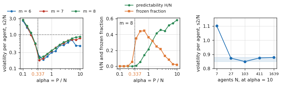
Fig. 1. Volatility per agent dips below the coin-flipping line (1.0) near alpha 0.4. Three memory lengths share the same dip. With alpha fixed, increasing the population sixty-fold (27 to 1639) keeps the reading within a 0.03 band; the 7-agent point is finite-size noise
A market with no data in it
The minority game contains no prices, no fundamentals and no news. It contains a population, a short public memory, and a rule for who gets paid. Everything the agents know is public. Under that condition the market should be unexploitable. The interest is in when, and how, that expectation fails.
Because it does fail, the word null has to be pinned down, and it is used in three senses below. Nothing here is a market in which no pattern exists. The library builds a market with no pattern planted in it, and whether that is a null for your test depends on three choices: the class of rules you search, the horizon they read, and the bar size you aggregate into. Each section says which it holds fixed.
The agent, and the one thing it decides
Each speculator holds a small fixed number of strategy tables. A table maps the last m outcomes, read as an m-bit word, to an action of plus or minus one. Tables are drawn at random when the population is created and never modified. What the agent learns is which table to trust: each carries a running score, and the agent plays the highest.
One convention has to be fixed, because the literature is not consistent about it. An outcome bit here is the sign of the excess demand, which is the side the majority took and therefore the side that lost; much of the literature writes the history as the winning side. The two differ by complementing every bit, which permutes the history words without merging any, so with random tables both conventions give the same distribution over everything measured below.
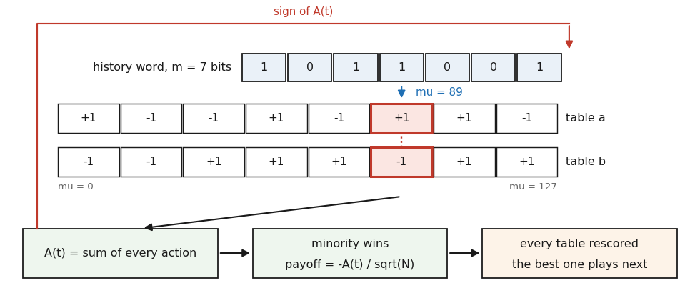
Fig. 2. The history word selects one column of every table, the actions are summed into excess demand, the minority is paid, and the sign of the demand, which is the majority side, becomes the newest history bit
This is weaker learning than it first appears, and the weakness is the point. The agent cannot invent a better rule, only reallocate trust across the handful it was born with, and every other agent is doing the same at the same time. The aggregate is a crowd effect, not a search for truth.
One structure carries every parameter of a population:
//+------------------------------------------------------------------+
//| MGConfig                                                         |
//|                                                                  |
//|  One population, two modes. Standard: every speculator trades    |
//|  every step, which is the model the phase transition is stated   |
//|  for. Grand canonical: a speculator sits out while its best      |
//|  score is below the benchmark, which is what produces returns.   |
//+------------------------------------------------------------------+
struct MGConfig
  {
   int               memory;          // m, bits of history each table reads
   int               speculators;     // adaptive agents, the N in alpha=P/N
   int               strategies;      // s, tables held per speculator
   int               producers;       // non-adaptive agents, one fixed table
   int               trendFollowers;  // injected bias, zero plants nothing
   double            trendProb;       // how often a follower follows
   double            epsilon;         // benchmark a speculator must beat
   double            initSpread;      // half width of the initial score noise
   double            depth;           // lambda, demand per unit log return
   bool              grandCanonical;  // false leaves every speculator active
   int               burnIn;          // steps run before anything is recorded
   int               steps;           // steps recorded
   ulong             seed;

   void              Defaults(void);
  };
Three fields deserve a note. producers are non-adaptive agents holding one fixed table each, and they are why a speculator has anything to exploit. trendFollowers are the injected bias, off at zero, so the detector can be pointed at a planted edge of a size you chose. epsilon is the benchmark a speculator's best table must beat, and does nothing unless grandCanonical is set.
A minority needs a strict majority to lose to, so with an even number of active agents the excess demand can land on zero and there is no minority to pay. Every population is sized through a helper that rounds to the nearest odd count:
//+------------------------------------------------------------------+
//| An odd population, because a minority needs a strict majority to |
//| lose to. With an even count the demand can land on zero, which   |
//| is a tie the model has no rule for                               |
//+------------------------------------------------------------------+
int OddAgents(const int memory, const double alpha)
  {
   double P = MathPow(2.0, (double)memory);
   int n = (int)MathRound(P / alpha);
   if(n < 3)
      n = 3;
   if(n % 2 == 0)
      n++;
   return(n);
  }
One step of the market
The step has four parts: read the history word, add up what everyone wants, pay the minority, and push the sign of the demand into the history. The first half collects the demand:
//+------------------------------------------------------------------+
//| The whole model. Read the history, add up what everyone wants,   |
//| pay the minority, push the sign of the demand into the history.  |
//| That sign names the majority, the complement of the winning side |
//| convention, so the words are relabeled and no statistic moves.   |
//+------------------------------------------------------------------+
void CMinorityGame::Run(void)
  {
   if(!m_built)
      return;

   int s = m_cfg.strategies;
   int P = m_P;
   double scale = 1.0 / MathSqrt((double)m_norm);
   int totalSteps = m_cfg.burnIn + m_cfg.steps;

   for(int t = 0; t < totalSteps; t++)
     {
      int mu = (int)m_mu;
      double A = 0.0;
      int active = 0;

      //--- speculators act on their current best table, and in grand
      //--- canonical mode only while that table is beating the benchmark
      for(int i = 0; i < m_cfg.speculators; i++)
        {
         int c = m_choice[i];
         if(m_cfg.grandCanonical && m_score[i * s + c] <= 0.0)
            continue;
         A += (double)m_specTab[(i * s + c) * P + mu];
         active++;
        }

      //--- producers are the reason there is anything to exploit: they
      //--- trade a fixed table forever and never learn from the outcome
      for(int j = 0; j < m_cfg.producers; j++)
         A += (double)m_prodTab[j * P + mu];

      //--- trend followers are the injected bias, and setting their
      //--- count to zero plants no pattern beyond the agents' own
      for(int j = 0; j < m_cfg.trendFollowers; j++)
        {
         int act;
         if(m_prevA != 0.0 && m_rng.NextDouble() < m_cfg.trendProb)
            act = (m_prevA > 0.0 ? 1 : -1);
         else
            act = m_rng.NextSign();
         A += (double)act;
        }
The speculator and producer loops index the same tables the same way. A producer's choice never changes, so it contributes a fixed pattern the speculators can learn to take the other side of. The trend follower loop is the only place an agent reads the previous outcome directly rather than through the history word.
The second half is where the learning happens:
      //--- every table is scored, not only the one that was played:
      //--- that virtual scoring is what makes the agent adaptive
      double coef = -A * scale;
      for(int i = 0; i < m_cfg.speculators; i++)
        {
         int base = i * s;
         int before = m_choice[i];
         int best = 0;
         double bv = 0.0;
         for(int a = 0; a < s; a++)
           {
            double u = m_score[base + a]
                       + coef * (double)m_specTab[(base + a) * P + mu];
            if(m_cfg.grandCanonical)
               u -= m_cfg.epsilon;
            m_score[base + a] = u;
            if(a == 0 || u > bv)
              {
               bv = u;
               best = a;
              }
           }
         m_choice[i] = best;
         if(best != before)
            m_moved[i] = 1;
        }

      //--- the freeze count is about the settled market, so the switch
      //--- flags are cleared once and only then start meaning anything
      if(t == m_cfg.burnIn)
         ArrayInitialize(m_moved, 0);

      //--- record only after the burn-in, so the learning transient
      //--- never lands in the statistics
      if(t >= m_cfg.burnIn)
        {
         int k = t - m_cfg.burnIn;
         m_A[k] = A;
         m_act[k] = (double)active;
         m_muSum[mu] += A;
         m_muCnt[mu] += 1.0;
        }

      //--- the sign of the demand names the majority, and that bit is
      //--- the public information every agent reads on the next step
      int bit;
      if(A > 0.0)
         bit = 1;
      else
         if(A < 0.0)
            bit = 0;
         else
           {
            //--- a tie has no minority. A fixed bit here would make zero
            //--- demand absorbing: no payoff, no learning, a dead history
            bit = (int)(m_rng.Next() >> 63);
           }
      m_mu = (((m_mu << 1) | (ulong)bit) & (ulong)(P - 1));
      m_prevA = A;
     }
  }
The scoring loop runs over every table an agent holds, not only the one it played. That is what makes the agent adaptive rather than lucky: a table that would have won gets credit, so it can rise to the top without being used. The payoff is the negative of total demand scaled by the square root of the population, the normalization the phase diagram is stated in.
Two details are easy to pass over. The switch flags are cleared when the burn-in ends, so the frozen fraction describes the settled market rather than the learning transient. And when demand lands on zero there is no minority, so the new history bit is drawn from the stream; without that draw zero demand is self-sustaining and the history word collapses to one value.
The two numbers the model is judged by
The first is the volatility per agent. The excess demand of N agents each playing plus or minus one has a variance that grows with N, so the useful quantity divides it out:
//+------------------------------------------------------------------+
//| Volatility per agent, a sample estimate whose expected value is  |
//| one for independent agents. A finite run scatters around that    |
//| rather than landing on it, so a reading is a statement about     |
//| coordination only once the scatter is allowed for                |
//+------------------------------------------------------------------+
double CMinorityGame::VolPerAgent(void) const
  {
   int n = ArraySize(m_A);
   if(n < 1)
      return(0.0);
   double ss = 0.0;
   for(int k = 0; k < n; k++)
      ss += m_A[k] * m_A[k];
   return(ss / (double)n / (double)m_norm);
  }
The scale is fixed by construction. If every agent flipped an independent coin the variance of the sum would be N in expectation, so this function has an expected value of 1.0. It is a sample estimate and will not land there, so the test allows a tenth either side rather than asserting the limit. Below one the population is coordinating better than chance; above one it is crowding onto the same side. The test measures 0.967 at alpha 89.5, the random agent limit approached rather than reached.
The second is the predictability, usually written H/N. Group every recorded step by the history word in force, take the mean demand inside each group, square it and average over the words actually visited:
//+------------------------------------------------------------------+
//| Predictability H/N: the mean demand conditional on the history   |
//| word, squared and averaged over the words this run actually      |
//| visited. Zero says the history tells a newcomer nothing, and it  |
//| is the order parameter that separates the two phases             |
//+------------------------------------------------------------------+
double CMinorityGame::Predictability(void) const
  {
   double h = 0.0;
   int seen = 0;
   for(int mu = 0; mu < m_P; mu++)
     {
      if(m_muCnt[mu] <= 0.0)
         continue;
      double mean = m_muSum[mu] / m_muCnt[mu];
      h += mean * mean;
      seen++;
     }
   if(seen == 0)
      return(0.0);
   return(h / (double)seen / (double)m_norm);
  }
Read it as one question: knowing nothing but the current history word, how well could a newcomer predict which side will be crowded? Zero is the strong form of efficiency inside this toy. A positive value says a pattern exists conditional on the state, and the whole population is leaving it there.
The divisor is a choice and deserves naming. This function averages over the words the run visited; the textbook definition averages over all P. The two agree exactly while every word is seen, and above the transition they cannot, because a short run over many words leaves some untouched and the visited-word average is then larger by the reciprocal of the coverage. The class reports both, with the coverage and the least-seen word's visit count. Measured at four points spanning the transition:
    predictability under both definitions, m = 8
       alpha   visited of P   minVisits   H/N visited    H/N all P
     0.1000      256 of 256          24       0.00160      0.00160
     0.5179      256 of 256           6       0.05419      0.05419
     2.6827      253 of 256           1       0.46003      0.45317
    10.0000      253 of 256           0       0.58415      0.57603
  [PASS] both definitions agree while every word is visited 256 of 256 words at alpha 0.1000, H/N 0.00160 and 0.00160
  [PASS] the order parameter turns on under the all-P definition too H/N over all P goes from 0.00160 to 0.57603
  [PASS] the visited-word average never understates the all-P one the two differ by a factor of 1.01 at alpha 10.00
Below the transition the coverage is complete and the question does not arise. Above it three words of 256 go unvisited, which moves the reading by one percent and moves no conclusion. It is kept because it need not stay small: the cross check's engine dump includes a configuration reaching only 20 of 32 words, where the two definitions read 0.965 and 0.603.
The phase diagram, and the collapse behind it
Sweeping alpha across two decades for three memory lengths gives the table Fig. 1 is drawn from:
     alpha    m=6 s2/N   m=7 s2/N   m=8 s2/N     m=8 H/N   m=8 frozen  m=8 minVisits
     0.1000     2.6001     2.7909     2.7565     0.00160       0.000          24
     0.1389     1.6451     1.7698     1.8401     0.00122       0.000          24
     0.1931     1.0156     0.9879     1.1487     0.00087       0.002          23
     0.2683     0.5329     0.5317     0.5617     0.00067       0.055          22
     0.3728     0.2267     0.1767     0.2074     0.00546       0.352          18
     0.5179     0.1851     0.1992     0.2253     0.05419       0.443           6
     0.7197     0.2276     0.2696     0.2731     0.14101       0.447           2
     1.0000     0.3015     0.3273     0.3437     0.21435       0.366           2
     1.3895     0.3296     0.4131     0.4044     0.32127       0.319           0
     1.9307     0.4866     0.5056     0.5048     0.41582       0.248           0
     2.6827     0.4939     0.5576     0.6005     0.46003       0.216           1
     3.7276     0.5975     0.6751     0.6616     0.44489       0.130           0
     5.1795     0.7063     0.7261     0.7743     0.51702       0.082           0
     7.1969     0.4764     0.7080     0.8441     0.54447       0.027           0
    10.0000     0.4696     0.7900     0.8705     0.58415       0.019           0
    m=6  volatility minimum at alpha = 0.5111  (s2/N = 0.1851)
    m=7  volatility minimum at alpha = 0.4313  (s2/N = 0.1767)
    m=8  volatility minimum at alpha = 0.4324  (s2/N = 0.2074)
  [PASS] m=6 minimum sits in the sub-unit decade      alpha_min 0.5111, grid step a factor of 1.39
  [PASS] m=7 minimum sits in the sub-unit decade      alpha_min 0.4313, grid step a factor of 1.39
  [PASS] m=8 minimum sits in the sub-unit decade      alpha_min 0.4324, grid step a factor of 1.39
  [PASS] the three minima collapse onto one alpha     spread 0.4313 to 0.5111, ratio 1.18
       geometric mean of the three minima: 0.4568
  [PASS] m=6 beats coin-flipping at the minimum       s2/N = 0.1851
  [PASS] m=6 crowding below the minimum               s2/N = 2.600 at alpha 0.100
  [PASS] m=7 beats coin-flipping at the minimum       s2/N = 0.1767
  [PASS] m=7 crowding below the minimum               s2/N = 2.791 at alpha 0.100
  [PASS] m=8 beats coin-flipping at the minimum       s2/N = 0.2074
  [PASS] m=8 crowding below the minimum               s2/N = 2.757 at alpha 0.100
    collapse at fixed alpha = 10, population growing
       m        N     s2/N
        6        7   1.1023
        8       27   0.8737
       10      103   0.8494
       12      411   0.8751
       14     1639   0.8783
  [PASS] s2/N is a function of alpha alone once N is large 0.8494 to 0.8783 over N = 27 to 1639
       N=7 reads 1.1023, which is where finite-size effects bite
Read the first column downwards. At alpha 0.1 there are ten times more agents than history words, each crowded by dozens holding correlated tables, and the volatility per agent is 2.6, worse than coin flipping. As alpha rises the crowd thins and the reading falls to 0.185 near alpha 0.5. Past that the population is too sparse to coordinate and the curve climbs back toward the random agent line.
The predictability column tells the mirror story. Below the transition it is 0.0016 or less, so the history word is worthless even at the market's most volatile. Above it predictability climbs past 0.5: calmer and far more predictable at once. The frozen fraction, the share of speculators that never switched table, peaks at 0.447 at the boundary. Three quantities turning together is the transition.
Now the discrepancy. The measured minima are 0.5111, 0.4313 and 0.4324 against the published 0.3374. That is not agreement, and the usual explanation, that a finite population smears a transition sharp only in the limit, is worth nothing until it carries a number. So the test refines the location on a narrow grid at five memory lengths, five populations from 117 agents to 1975:
    fine scan of the minimum, narrow grid, five populations
       9 points from 0.20 to 1.00, 2 seeds each
       m        N   alpha_min     s2/N   gap to alpha_c
        6      117      0.5501   0.1957           0.2127
        7      311      0.4113   0.1724           0.0739
        8      603      0.4255   0.2053           0.0881
        9     1147      0.4463   0.2361           0.1089
       10     1975      0.5184   0.3074           0.1810
  [PASS] the minimum sits in one narrow band across five populations 0.4113 to 0.5501 over N = 117 to 1975, ratio 1.34
  [PASS] that band sits above the published alpha_c at every population the closest is 0.4113 against 0.3374, a gap of 0.0739
       steps per history word fall from 125 at m=6 to 7 at m=10, which is why a larger N is not a sharper read
The gap does not close. It narrows from m equals 6 to 7 and widens again, while the depth of the minimum rises from 0.17 to 0.31. The last line says why: every run records 8000 steps, so a longer memory spreads one sample over twice as many words, and by m equals 10 each is seen about seven times. The larger populations are noisier readings, not better ones. What the five agree on is a band, 0.41 to 0.55, sitting entirely above the published value, so the supportable claim is that the minimum exists, depends on alpha rather than on m or N separately, and lands near but above 0.3374.
The collapse in the third panel is the sharper test, and the one that passes cleanly. Holding alpha at 10 while the population grows from 27 to 1639 leaves the volatility per agent between 0.849 and 0.878, which is what has to happen if alpha is the only control parameter, and it does not lean on the published constant. The reading is not 1.0 because that is the limit as alpha goes to infinity. The N equals 7 row reads 1.10, finite-size noise outside the asserted band.
Making the market behave like a market
A price series is only interesting if it looks like one. Cont's 2001 survey lists what essentially every liquid asset shows: returns near unpredictable in sign, far more extreme moves than a Gaussian, volatility clustered in time, and tails that thin as returns are aggregated. The plain minority game does not produce that list. It takes one more ingredient.
The option to sit out
In the plain game every speculator trades every step whether it expects to win or not. The grand canonical variant, due to Challet, Marsili and Zhang, adds a third option: stay out while the best table scores below a benchmark. That makes the number of active traders a variable, and a market whose participation breathes is one whose volatility clusters.
In the code it is two lines in the step loop: the continue that skips a speculator whose current table has fallen below zero, and the subtraction of epsilon from every score every step, which stops a table living on old winnings. The shipped configuration runs 1000 speculators against 512 producers and averages 97.6 active: the market is made by ten percent of the population, and which ten percent changes constantly.
The checklist, as numbers rather than impressions
The analyzer in StylizedFacts.mqh is free functions rather than a class, because each is a pure calculation on an array: the mean, the central moments, the autocorrelation at a lag, Ljung-Box with a chi-square tail, a Hill tail index, and the variance ratio. It lands in one flat structure:
//+------------------------------------------------------------------+
//| SFReport                                                         |
//|                                                                  |
//|  One reading of the checklist. Every field is a number the test  |
//|  script can assert on, so nothing here is left to be judged by   |
//|  eye from a chart.                                               |
//+------------------------------------------------------------------+
struct SFReport
  {
   int               n;                 // returns the report was built from
   double            mean;              // mean return
   double            stdev;             // population standard deviation
   double            skew;              // third moment, reported not tested
   double            excessKurtosis;    // zero is the Gaussian value
   double            acf1;              // lag-one return autocorrelation
   double            lbQ;               // Ljung-Box on the returns
   double            lbP;               // its upper tail probability
   double            absAcf1;           // lag-one absolute return acf
   double            absAcfMean;        // mean absolute acf over the window
   double            absLbQ;            // Ljung-Box on the absolute returns
   double            absLbP;            // its upper tail probability
   double            hillIndex;         // tail index of the absolute returns
   double            kurtAgg[5];        // kurtosis after aggregating
   double            varRatio[5];       // variance ratio at the same scales
   int               aggBlocks[5];      // the q of each scale
  };
Every field is a number the test script can assert on, which is why the structure exists. A chart of returns can be read as fat-tailed by one person and as normal by another; an excess kurtosis of 0.7214 against a control that reads negative 0.0041 cannot.
The variance ratio deserves its own note, because it is the one quantity here that looks past the autocorrelation window:
//+------------------------------------------------------------------+
//| Variance ratio at horizon q. One says the series diffuses like a |
//| random walk, above one says moves persist, and below one says    |
//| they are taken back. It is the cleanest single number for what a |
//| price does over a horizon longer than the autocorrelation window |
//+------------------------------------------------------------------+
double SFVarianceRatio(const double &x[], const int q)
  {
   if(q < 1)
      return(0.0);
   double v1 = SFMoment(x, 2);
   if(v1 <= 0.0)
      return(0.0);
   double agg[];
   SFAggregate(x, q, agg);
   if(ArraySize(agg) < 20)
      return(0.0);
   return(SFMoment(agg, 2) / (v1 * (double)q));
  }
Sum the returns in non-overlapping blocks of q, take the variance of the blocks, and divide by q times the variance of the step returns. A random walk gives one at every q; above one the price trends, below one it reverts. It matters because a series can be uncorrelated at lag one and still be strongly mean-reverting over five hundred steps, which is what the last sections turn on.
Running the checklist on independent noise, on the plain game and on the grand canonical game gives:
    independent noise      n 40000  sd 0.9983  skew +0.033  exkurt -0.0041
                           return acf1 -0.0078  LB p 0.302
                           |return| acf1 -0.0012  mean acf -0.0011  LB p 0.157
                           Hill index 6.17  kurt by scale -0.004 0.058 0.011 0.085 -0.000
                           variance ratio by scale 1.000 1.000 0.976 0.988 0.993
    plain game             n 40000  sd 0.04277  skew -0.010  exkurt +0.1572
                           return acf1 -0.0019  LB p 0.00337
                           |return| acf1 -0.0006  mean acf +0.0013  LB p 0.532
                           Hill index 6.23  kurt by scale 0.157 0.088 -0.022 0.006 -0.093
                           variance ratio by scale 1.000 0.992 0.987 0.973 0.881
    grand canonical game   n 40000  sd 0.003482  skew +0.013  exkurt +0.7214
                           return acf1 -0.0118  LB p 9.98e-17
                           |return| acf1 +0.0850  mean acf +0.0752  LB p 0
                           Hill index 3.97  kurt by scale 0.721 0.689 0.770 0.633 0.496
                           variance ratio by scale 1.000 0.984 0.972 0.926 0.773
       active speculators averaged 97.6 of 1000
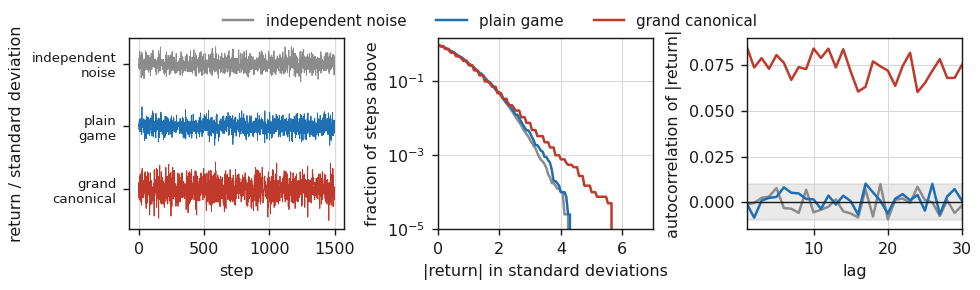
Fig. 3. The three series look alike as paths, separate in the far tail where the grand canonical game reaches past five standard deviations, and separate decisively in the autocorrelation of absolute returns, where only that game sits outside the noise band at every lag
The control comes out empty on all three counts, which licenses the rest of the reading: excess kurtosis of negative 0.0041, a Ljung-Box p of 0.302 on the returns and 0.157 on the absolute returns. If the analyzer manufactured structure, it would have manufactured it there.
The plain game gives an excess kurtosis of 0.157 and a mean absolute return autocorrelation of 0.0013, which is nothing. The grand canonical game gives 0.721 and 0.0752, a Ljung-Box p on the absolute returns underflowing to zero, and a Hill tail index of 3.97 against 6.17 for the control. Three to four is the figure usually reported for real daily returns.
The sign needs more care than it usually gets. The lag-one autocorrelations are negative 0.0019 and negative 0.0118, which look like nothing, but Ljung-Box on the same returns gives p equal to 0.00337 and 9.98e-17. Both reject independence outright, so writing that these games leave the sign unpredictable would be contradicted three lines above. What is true is an effect size, not an absence: those autocorrelations account for 0.0004 and 0.0139 percent of the return variance.
  [PASS] plain game: lag-one sign structure is negligible acf1 -0.0019, 0.0004% of the variance, Ljung-Box p 0.00337
  [PASS] grand canonical: lag-one sign structure is negligible acf1 -0.0118, 0.0139% of the variance, Ljung-Box p 9.98e-17
  [PASS] a one-step rule earns a trivial mean per step fading one step scores t +0.02 and +1.20, +0.0001 and +0.0060 of a standard deviation per step
The third line settles it, because a correlation is only worth a sentence once it is priced. Fading the previous step over all 40,000 returns scores a t of 0.02 on the plain game and 1.20 on the grand canonical one, and earns six thousandths of a standard deviation per step at best. The sign carries structure a test can find and a rule cannot use.
The benchmark is calibrated, and the band is narrow
Epsilon is a calibrated parameter, and it is worth saying so rather than dressing the choice up as a discovery. It was set by scanning against the checklist above and keeping the value whose output looks like a liquid asset, which makes that checklist a fitting criterion rather than an independent confirmation. What the scan does establish is how little room there is. Across a factor of four with everything else fixed, on 20,000 steps per point:
    benchmark scan, 20000 steps each
      eps      active     sd      exkurt   |r|acf   q25 kurt
      0.0006    102.5  6.941e-03   +28.666  +0.3979   +27.241
      0.0008     98.0  3.974e-03    +0.503  +0.0588    +0.156
      0.0012     96.7  3.265e-03    +0.223  +0.0361    +0.276
      0.0016     96.3  2.971e-03    +0.281  +0.0322    +0.012
      0.0024     95.4  2.722e-03    +0.246  +0.0175    +0.126
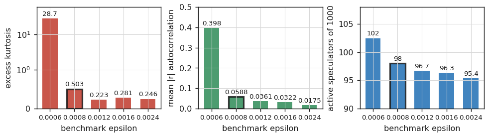
Fig. 4. Excess kurtosis falls from 28.7 to 0.503 between epsilon 0.0006 and 0.0008, and the outlined bar is the shipped setting; the third panel shows the participation moving by only seven agents across the whole scan
At 0.0006 the market is pathological: an excess kurtosis of 28.7 and a mean absolute return autocorrelation of 0.398 are not a liquid asset, and the kurtosis at the 25-step aggregation is 27.2, so the tails stay put instead of thinning. At 0.0024 it is nearly dead, at 0.246 and 0.0175. The realistic band is 0.0008, and the third panel shows why that is easy to miss: participation barely moves while the return distribution changes by a factor of fifty.
The test prints this scan on every run for that reason: changing the population or the producer count moves the band, and the scan is how a reader finds it again.
One limit on the section follows. Reproducing the stylized facts is necessary for a simulator to be worth using as a control, not sufficient: many processes with no economic content can be tuned to show fat tails and clustered volatility, and this one was. The parts not calibrated against what then checks them are the phase transition above and the double auction below.
Zero intelligence, and how much of the efficiency belongs to the rules
The second model is the one experiment whose benchmark can be computed exactly rather than simulated. Gode and Sunder gave each buyer a private redemption value and each seller a private cost, drawn uniformly, and let them trade in a continuous double auction with no strategy at all. Against what? Against the surplus a perfect central planner would reach, computable in closed form:
Against what? Against the surplus a perfect central planner would reach, which is computable in closed form from the drawn values:
//+------------------------------------------------------------------+
//| The surplus a planner would reach: match the highest value with  |
//| the lowest cost and keep pairing while the pair is worth it      |
//+------------------------------------------------------------------+
double CZeroIntelligence::MaxSurplus(double &eqPrice) const
  {
   double v[], c[];
   ArrayResize(v, ArraySize(m_value));
   ArrayCopy(v, m_value);
   ArrayResize(c, ArraySize(m_cost));
   ArrayCopy(c, m_cost);
   ArraySort(v);
   ArraySort(c);
   ArrayReverse(v);          // values descending, costs already ascending

   int nv = ArraySize(v), nc = ArraySize(c);
   int lim = (nv < nc ? nv : nc);
   double total = 0.0;
   int k = 0;
   while(k < lim && v[k] >= c[k])
     {
      total += v[k] - c[k];
      k++;
     }

   //--- the crossing is an interval, not a point, so report its middle
   if(k == 0)
     {
      eqPrice = 0.5 * (m_cfg.priceMin + m_cfg.priceMax);
      return(0.0);
     }
   double lo = c[k - 1];
   if(k < nv)
      lo = MathMax(lo, v[k]);
   double hi = v[k - 1];
   if(k < nc)
      hi = MathMin(hi, c[k]);
   eqPrice = 0.5 * (lo + hi);
   return(total);
  }
Sort the values downward and the costs upward, pair them off, and keep pairing while the pair is worth making. The total is the maximum gains from trade in that period, and the crossing is the competitive equilibrium price, reported as the middle of an interval because with discrete units the crossing is an interval.
The quoting rule itself is short. This is the part of RunOnePeriod that draws a quote and decides whether it trades, excerpted from a longer function that also handles the settlement and the bookkeeping:
   for(int q = 0; q < m_cfg.quotes && nb > 0 && ns > 0; q++)
     {
      //--- one agent is drawn from everyone still holding a unit
      ulong pick = m_rng.NextBounded((ulong)(nb + ns));
      bool isBuyer = ((int)pick < nb);
      int slot = (isBuyer ? (int)pick : (int)pick - nb);

      double price = 0.0;
      int hitB = -1, hitS = -1;

      if(isBuyer)
        {
         int i = m_liveB[slot];
         double top = (m_cfg.budgetConstrained ? m_value[i] : m_cfg.priceMax);
         double bid = m_cfg.priceMin
                      + m_rng.NextDouble() * (top - m_cfg.priceMin);
         if(asker >= 0 && bid >= bestAsk)
           {
            price = bestAsk;
            hitB = slot;
            hitS = asker;
           }
         else
            if(bid > bestBid)
              {
               bestBid = bid;
               bidder = slot;
              }
        }
      else
        {
         int j = m_liveS[slot];
         double bot = (m_cfg.budgetConstrained ? m_cost[j] : m_cfg.priceMin);
         double ask = bot + m_rng.NextDouble() * (m_cfg.priceMax - bot);
         if(bidder >= 0 && ask <= bestBid)
           {
            price = bestBid;
            hitS = slot;
            hitB = bidder;
           }
         else
            if(ask < bestAsk)
              {
               bestAsk = ask;
               asker = slot;
              }
        }
One line carries the experiment: the choice of top for a buyer and bot for a seller. With the budget constraint on, a buyer never bids above its value and a seller never asks below its cost, so no trade can destroy surplus. With it off, both quote across the full range and a trade can pair a buyer valuing the unit at 30 with a seller whose cost is 170.
The measurement:
    constrained    efficiency 0.9597  trades 32.9  price 99.28 vs equilibrium 99.17  dispersion 29.14
    unconstrained  efficiency -0.0228  trades 60.0  price 99.35  loss making trades 29.9
  [PASS] constrained surplus never exceeds the maximum 2815.82 of 2934.19
  [PASS] constrained traders are close to fully efficient efficiency 0.9597
  [PASS] removing the constraint costs efficiency     0.9597 vs -0.0228
  [PASS] only the unconstrained market trades at a loss 0.00 vs 29.93 per period
  [PASS] constrained prices sit near the equilibrium  99.28 vs 99.17
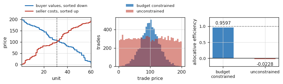
Fig. 5. The dotted line in the left panel is where supply crosses demand, the constrained trade prices concentrate near it while the unconstrained prices spread across the whole range, and the efficiency bars are measured against the surplus a planner could reach
Random traders under a budget constraint capture 96.0 percent of the surplus a planner could reach, at a mean trade price of 99.28 against an equilibrium of 99.17 and no trade destroying value, though prices scatter at a standard deviation of 29.14. Remove the constraint and efficiency falls to negative 0.0228: the market ends worse off than if it had not traded, with 29.9 of its 60 trades a period pairing a buyer and seller who should never have met.
The lesson transfers. Most of what looks like the intelligence of a market is the arithmetic of its matching rule, and a strategy that appears to profit from an efficient market may be profiting from a mechanism that would work without it.
The control no backtest on real data can offer
Now the payoff. With a market whose contents are known, a parameter search can be run against a series into which nothing was planted, and the resulting false discovery measured rather than argued about. The sense of null held fixed here is the first of the three: a lookback grid up to 20 steps, read at the step scale, against agents carrying a seven-bit memory.
Selecting on one half, paying on the other
The rule under test is the simplest one there is: sum the last L returns, go long if the sum is positive and short if it is negative, or do the reverse. One function scores it over a window:
//+------------------------------------------------------------------+
//| One rule evaluated over a half-open window. The signal is the    |
//| sum of the returns strictly before the step, kept as a sliding   |
//| window so a long lookback costs no more than a short one         |
//+------------------------------------------------------------------+
double EPEvaluate(const double &r[], const int from, const int to,
                  const int lookback, const int direction,
                  double &meanStep, int &bars)
  {
   meanStep = 0.0;
   bars = 0;
   int n = ArraySize(r);
   int start = (from > lookback ? from : lookback);
   int stop  = (to < n ? to : n);
   if(lookback < 1 || stop - start < 30)
      return(0.0);

//--- prime the window on the lookback returns that sit just before
//--- the first step being scored, and never on the step itself
   double signal = 0.0;
   for(int k = start - lookback; k < start; k++)
      signal += r[k];

   double s = 0.0, ss = 0.0;
   for(int t = start; t < stop; t++)
     {
      int pos = 0;
      if(signal > 0.0)
         pos = direction;
      else
         if(signal < 0.0)
            pos = -direction;
      double p = (double)pos * r[t];
      s += p;
      ss += p * p;
      bars++;
      signal += r[t] - r[t - lookback];
     }

   double m = s / (double)bars;
   double v = ss / (double)bars - m * m;
   meanStep = m;
   if(v <= 0.0)
      return(0.0);
   return(m / MathSqrt(v) * MathSqrt((double)bars));
  }
The signal is a sliding window, so a lookback of 1600 costs what a lookback of 5 costs. The position at step t is decided by information strictly older than t, and that ordering is the only thing between this function and a look-ahead.
The scan then does what an optimizer does, and keeps the evidence an optimizer throws away:
//+------------------------------------------------------------------+
//| Scan every lookback in both directions on the first part of the  |
//| series, take the single winner, and score it on the part it      |
//| never saw. The best and worst out-of-sample scores are kept too, |
//| so the gap up to the best is what hindsight would have supplied  |
//+------------------------------------------------------------------+
bool EPScanGrid(const double &r[], const int splitIndex,
                const int &lookbacks[], EPResult &res)
  {
   int n = ArraySize(r);
   int nL = ArraySize(lookbacks);
   if(splitIndex < 100 || n - splitIndex < 100 || nL < 1)
      return(false);

   res.lookback = 0;
   res.direction = 0;
   res.gridSize = 0;
   res.tIn = -1.0e300;
   res.tOut = 0.0;
   res.tOutBest = -1.0e300;
   res.tOutWorst = 1.0e300;
   res.meanIn = 0.0;
   res.meanOut = 0.0;
   res.barsIn = 0;
   res.barsOut = 0;

   for(int j = 0; j < nL; j++)
     {
      int L = lookbacks[j];
      for(int d = -1; d <= 1; d += 2)
        {
         double mIn = 0.0, mOut = 0.0;
         int bIn = 0, bOut = 0;
         double tIn = EPEvaluate(r, 0, splitIndex, L, d, mIn, bIn);
         double tOut = EPEvaluate(r, splitIndex, n, L, d, mOut, bOut);
         if(bIn < 1 || bOut < 1)
            continue;

         //--- the grid is antisymmetric: reversing the direction reverses
         //--- every trade, so half of it scores positive on any series
         res.gridSize++;
         if(tOut > res.tOutBest)
            res.tOutBest = tOut;
         if(tOut < res.tOutWorst)
            res.tOutWorst = tOut;

         //--- selection happens on the in-sample number only, which is
         //--- exactly the mistake the experiment is built to expose
         if(tIn > res.tIn)
           {
            res.tIn = tIn;
            res.tOut = tOut;
            res.lookback = L;
            res.direction = d;
            res.meanIn = mIn;
            res.meanOut = mOut;
            res.barsIn = bIn;
            res.barsOut = bOut;
           }
        }
     }

   return(res.gridSize > 0);
  }
Selection happens on the in-sample score alone, which is the mistake the experiment exposes. The scan also keeps the best and worst out-of-sample scores, because reversing direction reverses every trade: the grid is antisymmetric, so exactly half the variants score positive regardless of what the series contains, and a search reporting only its best result is guaranteed a positive number.
The power curve
Twenty independent markets are built at each of six bias levels, from no trend followers at all to 80 among 641 speculators. Each is split in half, the grid of 20 lookbacks in both directions is searched on the first half, and the winner scored on the second:
    followers    H/N      acf1     mean tIn   mean tOut    sd tOut   detected
            0   0.00021  -0.0057      1.702       0.284      0.972     0.0%
            5   0.00021  -0.0007      1.715       0.046      0.951     0.0%
           10   0.00018  -0.0033      1.694       0.331      0.934     5.0%
           20   0.00055  +0.0096      2.332       0.676      2.054    15.0%
           40   0.39861  +0.3842     31.825      31.983      2.677   100.0%
           80   1.85821  +0.6277     47.822      47.768      1.860   100.0%
  [PASS] null market: mean out-of-sample t            got 0.283987 want 0 +/- 1.17
  [PASS] null market: out-of-sample t has unit scale  standard deviation 0.972 over 20 markets
  [PASS] null market: detection rate stays near the false positive rate 0 of 20 markets crossed t = 2
  [PASS] in-sample selection always looks impressive  mean winning tIn on a null market 1.702
  [PASS] in-sample and out-of-sample part company on the null tIn 1.702 versus tOut 0.284
  [PASS] planting an edge moves the out-of-sample score 47.768 with 80 followers vs 0.284 with none
  [PASS] the detection rate rises from the smallest level to the largest 0 0 1 3 20 20 of 20
       twenty markets cannot order the three smallest levels, which is what the larger sample below is for
  [PASS] the largest planted edge is always found     20 of 20
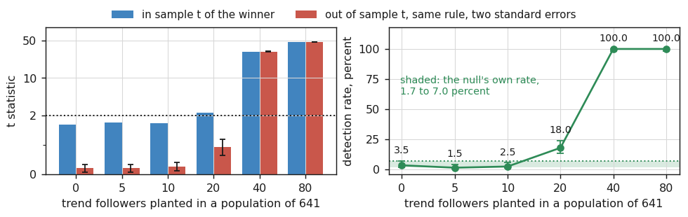
Fig. 6. Drawn from the 200 market confirmation below. On the null market the in-sample bar stands at 1.67 against an out-of-sample bar near zero, and the two only merge, and only clear the dotted t equals 2 line, once the planted edge is large enough. The shaded band on the right is the null market's own detection rate, and the three smallest levels sit inside it
On the null market the winning rule averages an in-sample t of 1.702, the kind of number that makes an optimizer report look worth trading. Out-of-sample it averages 0.284, at a standard deviation of 0.972 across twenty markets, and none of the twenty crossed t equals 2.
Twenty markets is enough to see that shape and not enough to bound any of it, so the whole curve is run again at ten times the sample, with a standard error on every mean and a Wilson interval on every rate:
    the same curve confirmed on a larger sample
    followers   mean tIn   mean tOut     se   sd tOut   detected   Wilson 95% on 200 markets
            0      1.672       0.205  0.066     0.932       3.5%     1.7% to   7.0%
            5      1.748       0.208  0.067     0.948       1.5%     0.5% to   4.3%
           10      1.729       0.257  0.068     0.957       2.5%     1.1% to   5.7%
           20      2.220       0.914  0.136     1.928      18.0%    13.3% to  23.9%
           40     31.233      31.491  0.184     2.598     100.0%    98.1% to 100.0%
           80     47.586      47.501  0.126     1.782     100.0%    98.1% to 100.0%
  [PASS] null market: the mean out-of-sample t is small but not zero 0.205 +/- 0.132, so 3.1 standard errors from zero
  [PASS] null market: the out-of-sample t keeps unit scale at scale standard deviation 0.932 over 200 markets
  [PASS] null market: the false discovery rate has a usable upper bound 7 of 200, Wilson 95% upper bound 7.0%
  [PASS] the gap between selection and payment survives the larger sample tIn 1.672 against tOut 0.205 on the null market
  [PASS] the smallest planted edges are indistinguishable from the null 1.5% and 2.5% against a null bounded by 7.0%
  [PASS] the curve separates from the null at twenty followers the 20 level starts at 13.3%, above the null's 7.0%
Two things that looked clean at twenty markets do not survive. The first is the out-of-sample score on the null: the standard deviation is 0.932, so the scale is right, but the mean is 0.205 with a standard error of 0.066, which is 3.1 standard errors above zero. It is not a draw from a standard normal. The next section shows why, measuring the generator as weakly anti-persistent at a t of negative 2.74 by a lookback of 20; selecting on the first half carries a little of that across, so a null defined by what the agents see is not a null for the selection procedure. The second is the power curve: at twenty markets the rate read 0, 0, 5, 15, 100, 100 and looked like a staircase, while at two hundred it reads 3.5, 1.5, 2.5, 18.0, 100 and 100, where the first three overlap each other and the null's own interval of 1.7 to 7.0 percent. That is a threshold between 10 and 20 followers, not a monotone rise, and a false discovery rate of 3.5 percent rather than zero.
The detector is not blind, which is the other half of the control. Plant 40 trend followers and predictability jumps from 0.0002 to 0.399, the out-of-sample t averages 31.5, and every one of the two hundred markets is detected; plant 80 and it averages 47.5. At 20 followers, three percent of the population, 18 percent are detected, so an edge that size is genuinely there and this search misses it four times in five.
Where the null stops being a null
This is the second sense of the word, and the one that limits the first. The agents read seven bits of history, so a rule that reads a comparable window sees what they see, and finds nothing. A rule that looks much further sees something else entirely, and the market stops being a null the moment the rule class is widened.
Ten markets, 40,000 steps each, and a momentum rule at nine lookbacks from 5 to 1600:
    out-of-sample t of a momentum rule, by lookback
      lookback      5      10      20      50     100     200     400     800    1600
      mean t     -0.61   -1.06   -2.74   -3.44   -4.70   -5.28   -6.20   -5.92   -5.91
    mean variance ratio at 500 steps: 0.1869
    scan winner: mean tIn 6.488, mean tOut 5.820, 10 of 10 detected
  [PASS] a rule the length of the agents' memory finds nothing t is -0.61 at lookback 5 and -1.06 at lookback 10
  [PASS] a much longer rule finds the mean reversion  momentum scores -5.92 at lookback 800, so fading it scores +5.92
  [PASS] the edge grows with the horizon              |t| goes from 2.74 at 20 to 5.92 at 800
  [PASS] the wide scan therefore does find an edge in the generator mean out-of-sample t 5.820, 10 of 10 markets
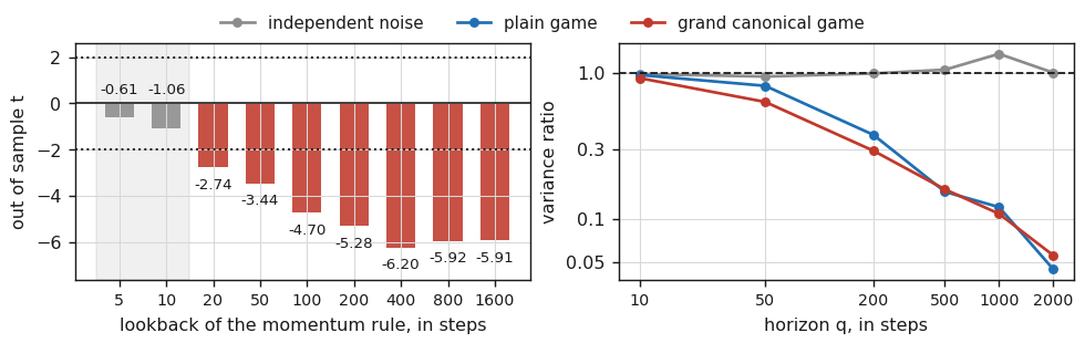
Fig. 7. Momentum scores nothing at the two shortest lookbacks, shaded on the left, and worse as the lookback grows until it flattens near negative 6 beyond lookback 400; the right panel shows why, with both games falling far below the random walk line while the control stays on it
At lookback 5 the momentum rule scores a t of negative 0.61 and at lookback 10 negative 1.06, the two shaded bars, and that is the sense in which the market has no edge. The decay is already underway by lookback 20, at negative 2.74, which is where the small positive bias in the previous section's null scan comes from. By lookback 800 it scores negative 5.92, so fading it scores positive 5.92, a reproducible out-of-sample edge in a market into which none was planted.
The right panel is the checklist run's own series read at six horizons:
    variance ratio at horizons 10 50 200 500 1000 2000
    independent noise        0.988   0.949   0.996   1.057   1.359   1.009
    plain game               0.973   0.819   0.377   0.153   0.120   0.045
    grand canonical game     0.926   0.635   0.293   0.159   0.108   0.056
The plain game falls to 0.153 at 500 steps and 0.045 at 2000, against a control that stays near one. The 0.1869 in the log above is that same quantity averaged over the ten markets. The price is strongly anti-persistent at long horizons: the population's coordination keeps pulling cumulative demand back toward zero, which over hundreds of steps reads as mean reversion. Nothing asked the model for it, and no rule reading seven bits can see it.
Important: a synthetic market is a control, not a customer. A strategy that survives the null here has cleared one failure mode, selection on an in-sample score, and nothing else. It has not been shown to hold on real prices, where the process changes, costs are real, and the participants are not agents reading a seven-bit word. Read a pass as one hypothesis surviving, not as evidence of profitability.
The simulated market as a tradable symbol
Everything above lives in arrays. To test a strategy on it the market has to become a symbol the Strategy Tester can open, which is what ABM_Symbol.mq5 does through MetaTrader's custom symbols. It builds one of the three markets, packs InpStepsPerBar model steps into each M1 bar, writes them, and reads them back to check they survived. The conversion has a trap in it:
//+------------------------------------------------------------------+
//| Turn the step returns into bars. The scale factor is chosen so   |
//| the finished bars carry the requested volatility, and is handed  |
//| back rather than recomputed, so the readback below can only ever |
//| be checking against the number that was actually used            |
//+------------------------------------------------------------------+
int MakeRates(const double &r[], MqlRates &rates[], const datetime base,
              const int periodSec, double &usedScale)
  {
   int steps = ArraySize(r);
   int bars = steps / InpStepsPerBar;
   usedScale = 0.0;
   if(bars < 2)
      return(0);

//--- the scale comes from the aggregated bar returns, not the step sigma
//--- times the root of the bar length: correlated steps break that rule
   double agg[];
   SFAggregate(r, InpStepsPerBar, agg);
   double sdBar = SFStdDev(agg);
   if(sdBar <= 0.0)
      return(0);
   double scale = InpBarSigma / sdBar;
   usedScale = scale;
   PrintFormat("    raw bar sigma %.6g scaled by %.6g to reach %.6g"
               " (square root of time would have given %.6g)",
               sdBar, scale, InpBarSigma,
               SFStdDev(r) * MathSqrt((double)InpStepsPerBar));

   ArrayResize(rates, bars);
   double price = InpStartPrice;
   int k = 0;

   for(int b = 0; b < bars; b++)
     {
      double open = price, hi = price, lo = price;
      for(int i = 0; i < InpStepsPerBar; i++)
        {
         price *= MathExp(r[k] * scale);
         if(price > hi)
            hi = price;
         if(price < lo)
            lo = price;
         k++;
        }
      rates[b].time = base + (datetime)(b * periodSec);
      rates[b].open = NormalizeDouble(open, InpDigits);
      rates[b].high = NormalizeDouble(hi, InpDigits);
      rates[b].low = NormalizeDouble(lo, InpDigits);
      rates[b].close = NormalizeDouble(price, InpDigits);
      rates[b].tick_volume = InpStepsPerBar;
      rates[b].spread = 0;
      rates[b].real_volume = 0;

      //--- rounding can push a close outside the range the same
      //--- rounding produced, so the envelope is repaired here
      rates[b].high = MathMax(rates[b].high,
                              MathMax(rates[b].open, rates[b].close));
      rates[b].low = MathMin(rates[b].low,
                             MathMin(rates[b].open, rates[b].close));
     }
   return(bars);
  }
The scale factor comes from the standard deviation of the aggregated bar returns, not the step deviation times the square root of the bar length, because step returns are correlated inside a bar. On the plain market the run below reports a raw bar sigma of 0.201 against the square root of time rule's 0.214. Rebuild the biased market and the same two numbers are 0.146 and 0.081, so the shortcut is out by a factor of 1.8.
Two smaller details earn their lines. Rounding the four prices independently can leave a close outside the high and low the same rounding produced, so the envelope is widened to enclose them. And the bars are written with a replace rather than a delete then an update, because a delete leaves the bar file in place and the terminal serves the old prices to the readback:
    model built: alpha 0.1997, volatility per agent 0.9772, predictability 0.00000
    removed a drift of 2.6001e-07 per step
    raw bar sigma 0.201443 scaled by 0.00198568 to reach 0.0004 (square root of time would have given 0.213857)
    wrote 20000 of 20000 bars from 2026.01.05 00:00 to 2026.01.18 21:19
  [PASS] every bar comes back out                 20000 of 20000
  [PASS] prices survive the round trip            0 bars differ
  [PASS] timestamps survive the round trip        0 bars differ
  [PASS] every bar is a well formed candle        0 bars malformed
  [PASS] stored closes carry the model's returns  worst gap 9.079e-06, rounding allows 3.636e-05
    one lot moves 10.00 per 100 points, and costs 1000.00 of margin; a 10,000 deposit therefore carries 10.0 lots
    price ran from 1.10000 to 1.10000, low 1.09709 high 1.10199
    bar sigma 0.000399965, acf1 -0.1229, variance ratio at 20/100/500 bars 0.164 0.042 0.010
Twenty thousand bars survive the round trip untouched, and the returns implied by the stored closes match the model's own to within 9.1e-06 where rounding allows 3.6e-05. The last line is the market's signature, and the lag-one autocorrelation of negative 0.123 in it is what the next section turns on.
Correct prices are not enough to make a symbol testable. The properties that decide what a position is worth are separate from the ones that decide what a bar looks like, and a symbol that gets them wrong will run a backtest to completion and report a profit of exactly zero:
   double point = MathPow(10.0, -(double)InpDigits);
   CustomSymbolSetInteger(name, SYMBOL_DIGITS, InpDigits);
   CustomSymbolSetInteger(name, SYMBOL_SPREAD_FLOAT, false);
   CustomSymbolSetInteger(name, SYMBOL_SPREAD, 0);
   CustomSymbolSetInteger(name, SYMBOL_TRADE_MODE, SYMBOL_TRADE_MODE_FULL);
//--- contract for difference, not foreign exchange: the forex mode parses
//--- a pair from the name, so ABM_MG cannot be valued as ABM against _MG
   CustomSymbolSetInteger(name, SYMBOL_TRADE_CALC_MODE,
                          SYMBOL_CALC_MODE_CFD);
   CustomSymbolSetInteger(name, SYMBOL_TRADE_EXEMODE,
                          SYMBOL_TRADE_EXECUTION_INSTANT);
   CustomSymbolSetInteger(name, SYMBOL_CHART_MODE, SYMBOL_CHART_MODE_BID);
   CustomSymbolSetDouble(name, SYMBOL_POINT, point);
   CustomSymbolSetDouble(name, SYMBOL_TRADE_TICK_SIZE, point);
//--- these modes charge margin on the whole notional without dividing by
//--- leverage, so a large contract refuses every order on a small deposit
   CustomSymbolSetDouble(name, SYMBOL_TRADE_CONTRACT_SIZE, InpContract);
   CustomSymbolSetDouble(name, SYMBOL_MARGIN_INITIAL, InpMarginPerLot);
   double tickValue = point * InpContract;
   CustomSymbolSetDouble(name, SYMBOL_TRADE_TICK_VALUE, tickValue);
   CustomSymbolSetDouble(name, SYMBOL_TRADE_TICK_VALUE_PROFIT, tickValue);
   CustomSymbolSetDouble(name, SYMBOL_TRADE_TICK_VALUE_LOSS, tickValue);
   CustomSymbolSetDouble(name, SYMBOL_VOLUME_MIN, 0.01);
   CustomSymbolSetDouble(name, SYMBOL_VOLUME_MAX, 100.0);
   CustomSymbolSetDouble(name, SYMBOL_VOLUME_STEP, 0.01);
Two of those lines carry the rest. The calculation mode has to be a contract for difference, not foreign exchange, because the forex mode reads a currency pair out of the name and ABM_MG resolves to a base of ABM against a profit currency of _MG. The difference modes charge margin on the whole notional without dividing by leverage, so a hundred thousand unit contract refuses every order on a ten thousand deposit.
Putting an Expert Advisor through it
A market whose answer is known is worth having only if you point your own optimizer at it. ABM_Demo.mq5 is the smallest Expert Advisor worth optimizing: one position at a time, long when the return over its lookback is positive and short when negative, with a direction input flipping between following the move and fading it.
//+------------------------------------------------------------------+
//| The signal is the return over the lookback, read from closed     |
//| bars only. Summing the last lookback bar returns telescopes to   |
//| a single ratio, so the whole rule is one logarithm               |
//+------------------------------------------------------------------+
int DesiredPosition(void)
  {
   double close[];
   ArraySetAsSeries(close, true);
   if(CopyClose(_Symbol, PERIOD_CURRENT, 1, InpLookback + 1, close)
      != InpLookback + 1)
      return(0);

   double signal = MathLog(close[0] / close[InpLookback]);
   if(signal > 0.0)
      return(InpDirection);
   if(signal < 0.0)
      return(-InpDirection);
   return(0);
  }
Summing the last few bar returns telescopes into a single logarithm, and reading it from bar 1 rather than bar 0 keeps the decision behind the information. Moving from the position held to the one wanted is the only other step:
//+------------------------------------------------------------------+
//| Move from the position held to the position wanted. A reversal   |
//| closes first and opens second, because netting accounts and      |
//| hedging accounts disagree about what a single opposite order     |
//| means and the two step form behaves the same on both             |
//+------------------------------------------------------------------+
void Reconcile(const int want)
  {
   int have = CurrentPosition();
   if(have == want)
      return;

   if(have != 0)
      g_trade.PositionClose(_Symbol);

   if(want > 0)
      g_trade.Buy(InpLots, _Symbol);
   else
      if(want < 0)
         g_trade.Sell(InpLots, _Symbol);
  }
A reversal closes before it opens rather than sending one opposite order, because netting and hedging accounts do not agree on what a single opposite order means. The magic number is read back before anything is closed, so the rule cannot adopt a position another program left on the chart. That runs once per closed bar:
//+------------------------------------------------------------------+
//| One decision per closed bar. Acting on the open of a bar whose   |
//| signal was built from bars strictly older than it is what keeps  |
//| this identical to the scan the library runs internally           |
//+------------------------------------------------------------------+
void OnTick(void)
  {
   datetime bar = (datetime)SeriesInfoInteger(_Symbol, PERIOD_CURRENT,
                                              SERIES_LASTBAR_DATE);
   if(bar == g_lastBar)
      return;
   g_lastBar = bar;

   Reconcile(DesiredPosition());
  }
Choosing the market to test on
Here is the third sense, and the one most easily missed: the same market can be a null at one bar size and not at another. Which market to build is therefore a measurement, not a preference. Thirty model steps per bar carries the previous section's long horizon mean reversion straight into the bar series, so what was a null at the step scale is no longer one. The same split at five aggregations shows where the boundary falls:
    a bar-level null needs acf1 near zero, variance ratios
    near one, and an out-of-sample t that does not follow
    the in-sample one

    market      s/bar    bars     acf1    vr20   vr100   L  d     tIn    tOut
    plain            1   20000  -0.0075   0.932  0.877   14 -1    +1.38   +0.31
    plain            2   20000  -0.0021   0.899  0.412   14 -1    +0.64   +1.53
    plain            5   20000  -0.0119   0.712  0.215   20 -1    +4.48   +7.76
    plain           10   20000  -0.0360   0.412  0.090   20 -1   +12.72  +12.59
    plain           30   20000  -0.1230   0.161  0.038   18 -1   +22.53  +22.66

    grand canonical   1   20000  -0.0016   0.850  0.439   20 -1    +4.98   +2.92
    grand canonical   2   20000  -0.0048   0.754  0.296   12 -1    +5.53   +4.35
    grand canonical   5   20000  -0.0271   0.524  0.214   16 -1   +11.23   +7.53
    grand canonical  10   20000  -0.0946   0.416  0.178    8 -1   +13.01  +10.22
    grand canonical  30   20000  -0.1638   0.335  0.155    2 -1   +17.53  +11.77
At thirty steps per bar the plain market hands a fading rule an out-of-sample t of 22.66. Finding that would be correct arithmetic, not a test of anything. At one step per bar the same market reads an autocorrelation of negative 0.008 and an out-of-sample t of 0.31 against an in-sample 1.38. That is the null, so the symbol both experiments run on is built with InpStepsPerBar at 1 rather than the default of 30: an autocorrelation near zero with variance ratios near one is what a bar-level null looks like.
What this optimizer finds in a market with nothing in it
Split the twenty thousand bars in half. Optimize the lookback from 2 to 20 in both directions on the first half, twenty parameter sets, then run the single best once on the second half. Every profit below is 0.10 lots on a 10,000 deposit at zero spread:
    ten lookbacks in both directions, first half only
      lookback  dir   trades    profit      PF   Sharpe
            18   -1      958    +42.54   1.118    +6.79
            12   -1     1128     +4.95   1.012    +0.79
            14   -1     1057     +3.37   1.008    +0.54
             8   -1     1380     -2.11   0.996    -0.34
            10   -1     1204     -3.30   0.993    -0.53
            16   -1      974     -5.58   0.986    -0.89
             4    1     2036     -9.29   0.985    -1.50
            20   -1      867     -9.99   0.973    -1.59
             2    1     2893    -22.07   0.972    -3.60
             6   -1     1595    -22.53   0.959    -3.63
            20    1      867    -24.69   0.936    -3.94
            16    1      974    -33.38   0.919    -5.00
             6    1     1595    -41.27   0.927    -5.00
            10    1     1204    -44.86   0.906    -5.00
            14    1     1057    -45.65   0.894    -5.00
            12    1     1128    -50.07   0.890    -5.00
             8    1     1380    -53.09   0.897    -5.00
             4   -1     2036    -72.15   0.891    -5.00
            18    1      958    -80.86   0.810    -5.00
             2   -1     2893    -93.65   0.886    -5.00
    3 of 20 parameter sets end the first half in profit

    the optimizer's choice, carried to the half it never saw
      lookback 18, fading, 958 trades in-sample
      in-sample     profit   +42.54   PF  1.12   Sharpe  +6.79
      out-of-sample profit   -53.86   PF  0.88   Sharpe  -5.00
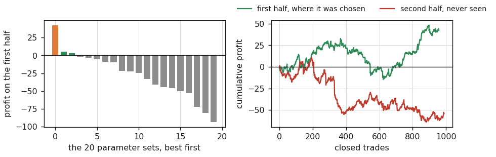
Fig. 8. Three of twenty sets end the first half in profit and the optimizer keeps the best of them, whose curve climbs to plus 42.54; the same rule on the untouched half falls to minus 53.86
A profit factor of 1.12 at a Sharpe of 6.79 is the kind of line that gets a strategy promoted to a demo account. On the half it never saw the same rule loses 53.86, at the reporting floor of negative 5. Nothing changed but which bars it was scored on, and nothing was ever there to find.
It is worse than that, because this symbol charges nothing: zero spread, no commission, no slippage. That isolates the selection effect and makes none of these figures a trading result. One lot moves 10.00 per 100 points, so at 0.10 lots a point is worth 0.01 and a round turn at a spread of S points costs S hundredths. The winning rule made 42.54 over 958 in-sample trades, or 4.4 points a trade, so a five point spread costs 47.90 and erases the whole in-sample profit before the second half is reached.
What an edge in the generator looks like, from the same seat
The market is a null only against rules shorter than the agents' memory. Widen the grid to lookbacks of 100 through 800 and the picture changes:
    eight longer lookbacks in both directions, same half
      lookback  dir   trades    profit      PF   Sharpe
           800   -1      396   +230.52   3.770   +36.85
           600   -1      417   +174.99   2.710   +27.85
           200   -1      401   +168.89   2.674   +26.88
           300   -1      419   +159.23   2.396   +25.33
           700   -1      407   +139.79   2.280   +22.22
           500   -1      387   +136.06   2.405   +21.63
           100   -1      412    +99.00   1.834   +15.74
           400   -1      415    +92.70   1.683   +14.78
           400    1      415   -109.30   0.542    -5.00
           100    1      412   -115.48   0.494    -5.00
           500    1      387   -151.54   0.376    -5.00
           700    1      407   -156.07   0.399    -5.00
           300    1      419   -175.99   0.379    -5.00
           200    1      401   -184.93   0.340    -5.00
           600    1      417   -191.67   0.336    -5.00
           800    1      396   -246.36   0.242    -5.00
    every one of the 8 fading sets is in profit, and none of the 8
    trend following ones is

    the optimizer's choice, carried to the half it never saw
      lookback 800, fading, 396 trades in-sample
      in-sample     profit  +230.52   PF  3.77   Sharpe +36.85
      out-of-sample profit  +139.68   PF  2.59   Sharpe +19.20
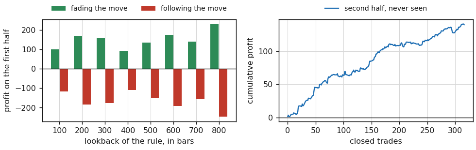
Fig. 9. Every one of the eight fading sets ends the first half in profit and every following set loses, and the winner goes on to earn plus 139.68 on the half it never saw
The same arithmetic separates the two results as sharply as the split does. The long rule took 317 trades on the half it never saw and made 139.68, which is 44 points a trade. It breaks even at a 44 point spread and keeps 108 of its 140 at 10, so this one has room the short grid's winner never had. That remains a statement about the generator: 44 points is about one bar's standard deviation here, far more forgiving than a real instrument.
The signature separates the two experiments. In the short grid one set of twenty was meaningfully positive and did not survive. In the long grid the direction input alone decides the sign, every fading set profits, every following set loses, and the winner keeps a profit factor of 2.59 out-of-sample. That is a property of the generator rather than of the search, and that distinction is the one real data cannot draw for you.
Neither result is a trading recommendation, and the second is not a trading edge at all. What it demonstrates is that a stable pattern inside a generator can be recovered by an honest out-of-sample procedure, which is a statement about the procedure. The anti-persistence it harvests belongs to agents coordinating on a seven-bit word. The transferable part is the method: run your strategy on a series into which nothing was planted, and you will know what a profit factor above one is worth.
Checking the engine from outside the terminal
A test script written by the same person who wrote the library shares its blind spots. The last piece of the project is a second implementation of the engine, in Python, that has to agree with the MQL5 original exactly.
Be clear about what that buys, because it is narrower than it sounds. Bit-for-bit agreement between two implementations of one specification establishes only that the specification was implemented twice without a transcription error. It says nothing about whether the model is economically sensible, whether the metrics are the right ones, or whether any of it resembles a real market: a flaw in the design reproduces as faithfully as the rest. Exact agreement is still worth insisting on, and it is not a general property of two IEEE 754 languages, which diverge through transcendental library functions, fused multiply-add, rounding modes and compilers. It holds here because the compared path is integer arithmetic plus addition, subtraction, multiplication and comparison in a fixed order on both sides, and where a transcendental appears the comparison carries a tolerance.
//+------------------------------------------------------------------+
//| One 64-bit output. The scrambler is the starred variant, which   |
//| passes BigCrush and costs two multiplies                         |
//+------------------------------------------------------------------+
ulong ABMRandom::Next(void)
  {
   ulong result = ABMRotl(s[1] * 5, 7) * 9;
   ulong t = s[1] << 17;
   s[2] ^= s[0];
   s[3] ^= s[1];
   s[1] ^= s[2];
   s[0] ^= s[3];
   s[2] ^= t;
   s[3] = ABMRotl(s[3], 45);
   return(result);
  }

//+------------------------------------------------------------------+
//| A double in [0,1). The top 53 bits are used because that is      |
//| exactly the mantissa, so the mapping is exact in both languages  |
//+------------------------------------------------------------------+
double ABMRandom::NextDouble(void)
  {
   return((double)(Next() >> 11) * (1.0 / 9007199254740992.0));
  }
The mapping to a double uses the top 53 bits, exactly the mantissa, so the conversion is exact on both sides. Every model draws from this one stream in a fixed order, so a replica that draws out of order produces a visibly different simulation rather than a subtly wrong one.
ABM_Export.mq5 writes one file holding every configuration next to every result, with doubles printed at seventeen significant digits so they round trip through text without loss. The cross check then does two things with it. It replicates the generator, the minority game, the double auction, the analyzer and the detector from the same rules and demands bit-for-bit equality. Then it recomputes the statistics with numpy, scipy and statsmodels, which reached those definitions by their own route, and that second layer would catch a formula faithfully transcribed but wrong:
SECTION 1  the generator, replicated
  [PASS] 64 raw words                                   64 values, 0 differ
  [PASS] 32 uniform doubles                             32 values, 0 differ
  [PASS] 64 bounded draws                               64 values, 0 differ
  [PASS] 64 signs                                       64 values, 0 differ
  [PASS] 32 normal draws                                worst relative difference 0.000e+00 over 32 draws
SECTION 2  the minority game, replicated
  [PASS] plain game: demand series                      300 values, 0 differ
  [PASS] plain game: volatility per agent               got 0.57333333333333336 want 0.57333333333333336  rel 0.000e+00 (tol 1e-15)
  [PASS] plain game: mean active                        got 31 want 31  rel 0.000e+00 (tol 1e-15)
  [PASS] plain game: history words visited              got 31 want 31
  [PASS] plain game: predictability over visited words  got 0.38075818089461244 want 0.38075818089461244  rel 0.000e+00 (tol 1e-15)
  [PASS] plain game: predictability over all P words    got 0.36885948774165578 want 0.36885948774165578  rel 0.000e+00 (tol 1e-15)
  [PASS] spread starting scores: demand series          300 values, 0 differ
  [PASS] spread starting scores: volatility per agent   got 0.47268817204301078 want 0.47268817204301078  rel 0.000e+00 (tol 1e-15)
  [PASS] spread starting scores: mean active            got 31 want 31  rel 0.000e+00 (tol 1e-15)
  [PASS] spread starting scores: history words visited  got 32 want 32
  [PASS] spread starting scores: predictability over visited words got 0.44930556594654514 want 0.44930556594654514  rel 0.000e+00 (tol 1e-15)
  [PASS] spread starting scores: predictability over all P words got 0.44930556594654514 want 0.44930556594654514  rel 0.000e+00 (tol 1e-15)
  [PASS] trend followers injected: demand series        300 values, 0 differ
  [PASS] trend followers injected: volatility per agent got 0.62940170940170936 want 0.62940170940170936  rel 0.000e+00 (tol 1e-15)
  [PASS] trend followers injected: mean active          got 31 want 31  rel 0.000e+00 (tol 1e-15)
  [PASS] trend followers injected: history words visited got 20 want 20
  [PASS] trend followers injected: predictability over visited words got 0.96506827109625082 want 0.96506827109625082  rel 0.000e+00 (tol 1e-15)
  [PASS] trend followers injected: predictability over all P words got 0.60316766943515676 want 0.60316766943515676  rel 0.000e+00 (tol 1e-15)
  [PASS] grand canonical: demand series                 300 values, 0 differ
  [PASS] grand canonical: volatility per agent          got 2.0602586206896554 want 2.0602586206896554  rel 0.000e+00 (tol 1e-15)
  [PASS] grand canonical: mean active                   got 134.66 want 134.66  rel 0.000e+00 (tol 1e-15)
  [PASS] grand canonical: history words visited         got 32 want 32
  [PASS] grand canonical: predictability over visited words got 0.013338738057103722 want 0.013338738057103722  rel 0.000e+00 (tol 1e-15)
  [PASS] grand canonical: predictability over all P words got 0.013338738057103722 want 0.013338738057103722  rel 0.000e+00 (tol 1e-15)
SECTION 3  the double auction, replicated
  [PASS] budget constrained: trade prices               49 values, 0 differ
  [PASS] budget constrained: realized                   got 834.4068387207656 want 834.4068387207656
  [PASS] budget constrained: maximum                    got 864.8022735467996 want 864.8022735467996
  [PASS] budget constrained: equilibrium                got 96.00100744723787 want 96.00100744723787
  [PASS] budget constrained: trades                     got 9.8 want 9.8
  [PASS] budget constrained: losing                     got 0.0 want 0.0
  [PASS] budget constrained: efficiency                 got 0.9648527348322365 want 0.9648527348322365
  [PASS] budget constrained: surplus never exceeds the maximum 834.406839 of 864.802274
  [PASS] unconstrained: trade prices                    100 values, 0 differ
  [PASS] unconstrained: realized                        got -464.67011644920075 want -464.67011644920075
  [PASS] unconstrained: maximum                         got 807.4813936523338 want 807.4813936523338
  [PASS] unconstrained: equilibrium                     got 88.70814131013566 want 88.70814131013566
  [PASS] unconstrained: trades                          got 20.0 want 20.0
  [PASS] unconstrained: losing                          got 12.0 want 12.0
  [PASS] unconstrained: efficiency                      got -0.5754561282798639 want -0.5754561282798639
  [PASS] unconstrained: surplus never exceeds the maximum -464.670116 of 807.481394
SECTION 4  the analyzer, replicated
  [PASS] series length                                  got 4000 want 4000
  [PASS] mean                                           got 3.141534391534391e-05 want 3.141534391534391e-05
  [PASS] standard deviation                             got 0.005054582422473009 want 0.005054582422473009
  [PASS] excess kurtosis                                got 0.1590071861918947 want 0.1590071861918947
  [PASS] lag-one return autocorrelation                 got -0.003882466746185918 want -0.003882466746185918
  [PASS] lag-one absolute autocorrelation               got 0.03367944211512192 want 0.03367944211512192
  [PASS] absolute autocorrelation profile               20 values, 0 differ
  [PASS] mean absolute autocorrelation                  got 0.021027527940826372 want 0.021027527940826372
  [PASS] Ljung-Box Q on the returns                     got 25.57447105036661 want 25.57447105036661
  [PASS] Ljung-Box Q on the absolute returns            got 52.70691669382414 want 52.70691669382414
  [PASS] Hill tail index                                got 5.88111981741711 want 5.88111981741711  rel 0.000e+00 (tol 1e-14)
  [PASS] kurtosis aggregated over 1 steps               got 0.1590071861918947 want 0.1590071861918947
  [PASS] variance ratio at 1 steps                      got 1.0 want 1.0
  [PASS] kurtosis aggregated over 2 steps               got 0.1577833066414156 want 0.1577833066414156
  [PASS] variance ratio at 2 steps                      got 0.974716646911691 want 0.974716646911691
  [PASS] kurtosis aggregated over 5 steps               got 0.4062521002451045 want 0.4062521002451045
  [PASS] variance ratio at 5 steps                      got 0.9487140032352153 want 0.9487140032352153
  [PASS] kurtosis aggregated over 10 steps              got -0.07049952952287875 want -0.07049952952287875
  [PASS] variance ratio at 10 steps                     got 0.934798480394314 want 0.934798480394314
  [PASS] kurtosis aggregated over 25 steps              got -0.30669299428955066 want -0.30669299428955066
  [PASS] variance ratio at 25 steps                     got 0.7611441621201054 want 0.7611441621201054
SECTION 5  the analyzer, against numpy scipy and statsmodels
  [PASS] excess kurtosis vs scipy                       got 0.15900718619189469 want 0.15900718619174281  rel 9.552e-13 (tol 1e-09)
  [PASS] skewness vs scipy                              got 0.011027923486822732 want 0.011027923486822805  rel 6.607e-15 (tol 1e-09)
  [PASS] standard deviation vs numpy                    got 0.005054582422473009 want 0.0050545824224730446  rel 7.036e-15 (tol 1e-12)
  [PASS] lag-one autocorrelation vs numpy               got -0.003882466746185918 want -0.0038824667461859774  rel 1.530e-14 (tol 1e-09)
  [PASS] Ljung-Box Q vs statsmodels                     got 25.574471050366611 want 25.574471050365773  rel 3.278e-14 (tol 1e-09)
  [PASS] Ljung-Box p vs statsmodels                     got 0.18033006741055593 want 0.18033006741067398  rel 6.546e-13 (tol 1e-09)
  [PASS] chi-square tail vs scipy                       got 8.974028472430047e-05 want 8.9740284724344706e-05  rel 4.929e-13 (tol 1e-09)
SECTION 6  the detector, replicated
  [PASS] grid size                                      got 24 want 24
  [PASS] winning lookback                               got 12 want 12
  [PASS] winning direction                              got -1 want -1
  [PASS] in-sample t of the winner                      got 1.4688883457816135 want 1.4688883457816135
  [PASS] out-of-sample t of the winner                  got 1.8121801330070035 want 1.8121801330070035
  [PASS] best out-of-sample over the grid               got 1.9123630301646217 want 1.9123630301646217
  [PASS] worst out-of-sample over the grid              got -1.9123630301646217 want -1.9123630301646217
  [PASS] the selected rule lies inside the grid range   -1.9124 <= 1.8122 <= 1.9124
  [PASS] no in-sample score beats the one that was selected winning tIn 1.4689
  [PASS] the grid is antisymmetric in the direction     best +1.9124 worst -1.9124, 12 of 24 score positive
-----------------------------------------------------------
  83 passed, 0 failed
=== ALL PASS ===============================
The tolerances are the interesting part. Everything the engine produces compares at exactly zero difference, including both predictability definitions, and the configuration reaching only 20 of 32 history words is the one that would expose a divisor copied across by eye. The comparisons against the outside libraries carry a relative tolerance near 1e-09, because a chi-square tail from a continued fraction and one from scipy's incomplete gamma need not agree in the last bit; the largest disagreement measured is 9.6e-13.
Conclusion
The library produces a market you can point a strategy at while knowing what was put into it, and the double auction inside it reproduces the Gode and Sunder result to within four percent of the planner's surplus.
Five findings are worth carrying away. The plain minority game does not produce the stylized facts; the option to sit out does. The benchmark switching it on is a knife edge, moving excess kurtosis from 28.7 to 0.503 in one step of the scan while participation barely twitches. The null is a null only up to the agents' memory, only at the aggregation you build bars from, and only for the rules you search. On it an optimizer still hands you a profit factor of 1.12, which becomes minus 53.86 on the next bars and would not have survived half a pip of spread. And it is not perfectly null even for this grid: over 200 markets its out-of-sample t averages 0.205 rather than zero.
- A minority game with producers, trend followers and a grand canonical mode, which locates its own volatility minimum unaided and measures the gap to the published one across five populations
- A Gode and Sunder double auction scored against a planner's surplus computed exactly rather than simulated
- An analyzer that turns the Cont checklist into pass or fail numbers, and a scanner that keeps the evidence an optimizer throws away, with its false discovery rate measured over 200 markets rather than asserted
- A tradable custom symbol, an Expert Advisor to optimize on it, and a Python replica that matches the engine bit-for-bit
| # | Filename | Type | Description |
|---|---|---|---|
| 1 | ABMRandom.mqh | Include | The xoshiro256** stream seeded through splitmix64, with uniform, bounded, sign and normal draws |
| 2 | MinorityGame.mqh | Include | The minority game: strategy tables, the step loop, producers, trend followers, the grand canonical mode, and the order parameters |
| 3 | ZeroIntelligence.mqh | Include | The continuous double auction with the budget constraint as a switch, and the planner surplus computed exactly |
| 4 | StylizedFacts.mqh | Include | Moments, autocorrelation, Ljung-Box with a chi-square tail, Hill tail index, aggregation and variance ratios |
| 5 | EdgeProbe.mqh | Include | The parameter scan: one rule scored over a half-open window, and a grid split into selection and evaluation halves |
| 6 | ABM_Test.mq5 | Script | Eighty-two assertions across eight sections, including the phase sweep, the checklist, the benchmark scan and the power curve |
| 7 | ABM_Symbol.mq5 | Script | Builds one of the three markets as a custom symbol and reads the bars back to verify them |
| 8 | ABM_Export.mq5 | Script | Writes every configuration and every result at seventeen significant digits for the cross check |
| 9 | ABM_Demo.mq5 | Expert Advisor | The momentum or fading rule as a tradable Expert Advisor, for optimizing against the synthetic symbol |
| 10 | abm_crosscheck.py | Python | Replicates the engine bit-for-bit and recomputes the statistics against numpy, scipy and statsmodels |
| 11 | MQL5.zip | Archive | Archive with all project files in their subfolders; unpack it into the terminal data directory and every file lands in its required location |
Warning: All rights to these materials are reserved by MetaQuotes Ltd. Copying or reprinting of these materials in whole or in part is prohibited.
This article was written by a user of the site and reflects their personal views. MetaQuotes Ltd is not responsible for the accuracy of the information presented, nor for any consequences resulting from the use of the solutions, strategies or recommendations described.

 Try/Catch style in MQL5: Bringing Modern Error Management to Algorithmic Trading
 Adaptive Trade Management in MQL5: Building a Broker-Aware, Deterministic, and Explainable Exit Engine
 Nonlinear OHLC Features Derived from Elliptic Curves
 The MQL5 Standard Library Explorer (Part 17): Building a Reusable Portfolio Manager with CArrayObj

- Free trading apps
- Over 8,000 signals for copying
- Economic news for exploring financial markets
You agree to website policy and terms of use