MetaTrader 5 Machine Learning Blueprint (Part 23): Feature Screening

Table of Contents

1. Introduction
2. Why a Feature Screen Needs Its Own Calibrated Null
3. The Three-Gate Pipeline
4. Gate 1: Stationarity, Running ADF and KPSS Together
5. Gate 2: Entropy, Uniform Binning, Not Quantile
6. Gate 3: Mutual Information and the Family-Wise Correction
7. Running the Screen on EURUSD H1
8. What the Result Does Not Show
9. Conclusion
10. Attached Files

Introduction

Every article in this series up to Part 19 has assumed the feature matrix already exists. A candidate column shows up, gets fractionally differenced or z-scored, and enters the model. Nothing in that pipeline asks whether the column deserved to be there. The usual first step (correlation, or a quick model with an importance score) implicitly uses a null hypothesis that is wrong for financial data. The obvious fix is a permutation test: shuffle the target, recompute the statistic, and see how often the shuffled version beats the real one. That fix can also be wrong, and this article spends its second section measuring how wrong, on EURUSD data rather than on a textbook example.

The failure mode is specific. Ordinary shuffling of a target series assumes every observation is exchangeable with every other one. A twenty-bar forward return is not exchangeable with anything: bar t and bar t+1 share nineteen of their twenty return contributions. An independent permutation destroys that overlap, so the null describes a different and easier estimation problem than the one the feature faces. In the configuration measured below (a persistent synthetic feature against the real overlapping EURUSD target), naive shuffling rejected a true null in all 200 trials at a nominal 5% level. The same section shows that the size of the distortion depends on the feature's persistence, the label overlap, and the test statistic, so it is not a fixed property of shuffling.

This article implements afml.screening with three gates: stationarity, entropy, and mutual information. The gates are not three versions of one idea. Gate 1 runs two formal hypothesis tests (ADF and KPSS) per feature. Gate 2 is a descriptive filter with no null and no p-value. Gate 3 is the only gate that draws its reference distribution from the resampling layer of Section 2, and the only one that can select a feature. Every number below comes from the H1 EURUSD dataset used across this series (42,584 aligned bars, 2018 through 2024) screened against a real twenty-bar forward return. One of the nine candidate columns is synthetic, and it is disclosed as such where it appears.

This article is Part 23 of the series. It starts a four-part sequence on degradation avoidance: Part 23 screens features; Part 24 quantifies sequence risk; Part 25 replaces the sequential test; Part 26 tests process robustness. The prerequisite from earlier in the series is Part 1's treatment of look-ahead bias in fractional differentiation. The stationarity gate here is restricted to raw candidate features and must not be run on fractionally differenced output, for the reasons given in Section 4.

Why a Feature Screen Needs Its Own Calibrated Null

Take a feature that is independent of the target by construction: an AR(1) process with φ = 0.95, generated from a random-number stream that has never seen the target series. Pair it with a real target, the twenty-bar forward log return on EURUSD H1, taken as a random contiguous window of 5,000 bars on each trial. The test statistic is the normalized mutual information with Miller-Madow correction, the same statistic Gate 3 uses. Every rejection is a false positive, so a correctly calibrated test should reject close to the nominal 5% of the time.

Four nulls are compared. The first, naive_shuffle, applies an independent random permutation to the target. The second, circular_shift, rotates the target by a random offset, which preserves every lag-k autocorrelation of the target except at the wrap-around seam. The third adds period=24 to the rotation, which restricts offsets to whole multiples of 24 bars and so keeps every observation at its original hour of day. The fourth, stationary_bootstrap, resamples the target in geometric blocks with mean length L. Each trial uses 200 resamples.

Scheme	Trials	Rejection rate	95% interval
naive_shuffle	200	100.0%	98.2% to 100.0%
circular_shift	1,000	4.1%	3.0% to 5.5%
circular_shift, period=24	1,000	5.4%	4.1% to 7.0%
stationary_bootstrap, L=100	1,000	9.3%	7.6% to 11.3%

Rejection rate of a true null by resampling scheme and block length

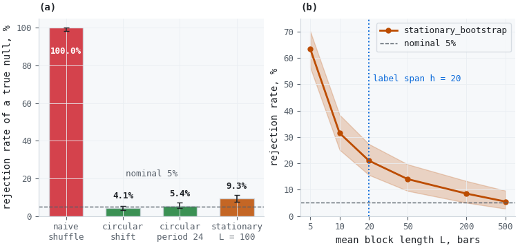
Figure 1. 2-panel illustration of null calibration on a true null

• Panel (a): false-positive rate of the mutual-information test under four nulls, with exact 95% intervals and the nominal 5% level dashed.
• Panel (b): false-positive rate of the stationary bootstrap as the mean block length L grows, 200 trials per point; the dotted line marks the twenty-bar label span.

Reading the calibration

naive_shuffle rejected a true null in every trial. circular_shift and circular_shift with period=24 both have intervals that contain 5%. The stationary bootstrap is oversized at L = 100, and its size depends strongly on L: it rejects 63.5% of true nulls at L = 5, 21.0% at 20, 8.5% at 200, and 5.5% at 500. In this configuration the bootstrap approaches nominal size only when the mean block is roughly 25 times the label span, so a block length must be chosen, measured, and reported with every result that uses the scheme. The module raises an error if mean_block is not supplied.

The statistic matters as well. Replacing normalized mutual information with absolute Pearson correlation on the same design (200 trials) gives 58.0% for naive_shuffle, 3.5% for circular_shift, and 4.5% for stationary_bootstrap at L = 100. The ordering of the schemes is the same. The size of the naive-shuffle failure is not.

Where the failure comes from

Where the naive-shuffle failure comes from, and a power baseline for rolling stationarity

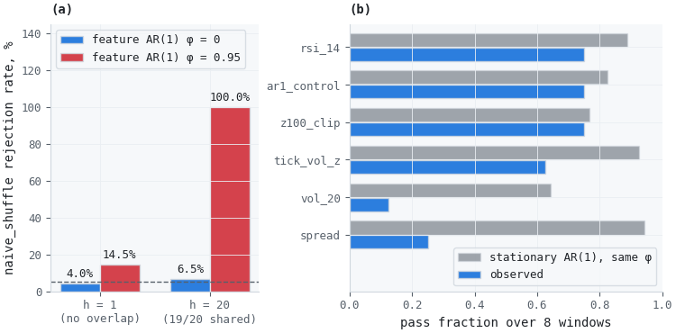
Figure 2. 2-panel illustration of naive-shuffle size and rolling-stationarity power

• Panel (a): false-positive rate of naive_shuffle for a white-noise and a persistent feature, against a non-overlapping and an overlapping target.
• Panel (b): fraction of eight windows returning a stationary verdict for each continuous candidate (blue) against the fraction a stationary AR(1) series of the same persistence returns (grey); discussed in Section 7.

Panel (a) separates the two ingredients. With a white-noise feature, naive_shuffle rejects 4.0% of true nulls against a non-overlapping target and 6.5% against the overlapping one. With a persistent feature it rejects 14.5% against the non-overlapping target and 100% against the overlapping one. The failure therefore needs a persistent feature, and label overlap turns a moderate distortion into a total one. The rate does not fall with sample size: it stays at 100% at both 2,000 and 10,000 bars. The shuffled null understates the sampling variability of a statistic computed between two serially dependent series, and more data does not repair that. The 14.5% cell is a separate effect that this study does not decompose. circular_shift sits between 3.0% and 5.0% in all four cells.

One limit of rotation needs stating. A rotation preserves the target's own dependence and its sequence of volatility regimes, but it breaks the alignment between the target and the calendar. If the feature and the target share an intraday or weekly seasonal component, a plain rotation will report that shared component as dependence. The synthetic feature here has no seasonality, so plain rotation and period=24 agree. They do not have to agree on a real feature, and Section 7 shows a case where the distinction matters. On calendar-indexed data with missing bars, period=24 preserves alignment in bar counts, not in wall-clock hours.

This is the reason afml.screening.permutation exists as a module in its own right rather than as a private helper inside each gate. Gate 3, and the monitoring work in Parts 24 and 25, draw their nulls from it. A miscalibrated scheme here is inherited everywhere the module is reused.

The Three-Gate Pipeline

The pipeline runs three gates in a fixed order, and the order is a claim about cost, transportability, and power.

Gate	Function	Statistical status	Can it select?
1. Stationarity	stationarity_gate	ADF and KPSS hypothesis tests at level α; no resampled null	No, rejects only
2. Entropy	entropy_screen	Descriptive thresholds; no null, no p-value	No, rejects only
3. Mutual information	mi_screen	Resampled joint null with Westfall-Young correction	Yes, the only gate that can

Stationarity runs first, but not because a non-stationary feature breaks the resampling null. With the target resampled and the feature held fixed, the validity of the Gate 3 null depends on the target's properties, and Section 7 shows a unit-root price column producing a well-formed null. There are two other reasons. A mapping estimated across a drifting feature distribution is not the mapping the model meets out of sample, which is a transportability problem. A drifting feature binned on a uniform grid also has a much wider mutual-information null (the raw price column in Section 7 has a null mean about seven times that of RSI), which costs power in its own test and, under a maximum-statistic correction, in every other test in the family.

Entropy runs second because it is O(N) and its verdict is one-directional. By the bound I(X; Y) ≤ H(X), a continuous feature that barely varies on its grid has little information to offer any target, and rejecting it saves permutation budget for candidates that might have more. Mutual information runs last because it costs n_perm full evaluations and is the only gate that can endorse a feature.

The error accounting needs care, because the gates differ. Gate 1 is two hypothesis tests per feature with their own error rates, and nothing corrects them across features. They can only remove features. A false rejection at Gate 1 or Gate 2 loses a feature, and it cannot create a false selection, because nothing is selected without clearing Gate 3. Whether the filters distort Gate 3's family-wise error rate turns on one property: both filters are functions of the features alone and never see the target. With the target resampled and the features fixed, the filter outcome is identical in every replicate, which is the independent-filtering condition of Bourgon, Gentleman, and Huber (2010). Correcting only over the survivors is then valid. The condition fails if a threshold is tuned after looking at Gate 3 output, because the filter then depends on the target through the researcher. It also holds only approximately under bar_permute, where features are recomputed on each permuted series but the filters are applied once, to the real features.

Set min_entropy, max_modal_occupancy, and alpha once, before looking at any result, and do not revisit them per feature set.

from afml.screening import screen_features

report = screen_features(
    features, target,
    alpha=0.05,
    min_entropy=0.5,
    max_modal_occupancy=0.5,
    scheme="circular_shift",
    scheme_kwargs={"period": 24},   # keep hour-of-day alignment
    n_perm=500,
    seed=0,
)
print(report)             # ScreeningReport(k/n selected, m tested at gate 3, effective_tests=...)
report.summary()          # one row per feature, gate-by-gate outcome
report.settings           # thresholds, scheme and scheme arguments behind every p-value

screen_features returns a ScreeningReport: the per-gate diagnostic tables, the list of selected features, a dictionary mapping every rejected feature to the gate that rejected it, the settings behind the p-values, and effective_tests, the independent-test equivalent of the family that reached Gate 3, read off the joint resampled null rather than assumed. Section 7 runs this against real EURUSD candidates.

Gate 1: Stationarity, Running ADF and KPSS Together

The module this gate supersedes, afml.features.stationary.is_stationary, runs the augmented Dickey-Fuller test alone, with the lag order fixed at one, and returns a boolean. A single test fails in two directions. ADF's null hypothesis is a unit root, so failing to reject is absence of evidence against a unit root, not evidence of stationarity. A persistent but stationary feature on a short sample fails to reject and is discarded. In the other direction, ADF rejecting says only that the series is not a pure random walk. It cannot see departures from short-memory level stationarity such as level shifts, slowly varying variance, or long memory, so those features pass. Section 7 shows the second failure on real data: the ADF-only gate rejects one of nine columns and passes the three that KPSS flags.

KPSS inverts the null: its null hypothesis is stationarity, and it rejects when the evidence points away from it. Running both against the same series and reading the pair jointly separates four outcomes that a single test conflates:

ADF	KPSS	Verdict
rejects	does not reject	stationary
does not reject	rejects	unit_root: route to fractional differentiation
rejects	rejects	conflicting, or trend_stationary if a linear-trend re-run resolves it
does not reject	does not reject	inconclusive: insufficient power

The third row is not a single process class. Under the level specification, both tests rejecting means the series is neither a random walk nor short-memory stationary around a fixed mean. Candidates include a deterministic trend, a structural break in the mean, long memory, and strong heteroskedasticity, each of which can inflate the KPSS statistic. assess_stationarity therefore re-runs both tests with a linear trend. If ADF rejects and KPSS does not under that specification, the verdict is trend_stationary. Otherwise it stays conflicting, and the gate does not claim to know which mechanism is responsible.

The specification is fixed so that verdicts are reproducible. ADF uses a constant only, with the lag order chosen by AIC up to the Schwert ceiling 12(n/100)0.25. KPSS tests level stationarity with a Newey-West long-run variance and the data-dependent bandwidth of Hobijn, Franses, and Ooms (1998). Both use the same α. They are formal hypothesis tests with their own error rates: at α = 0.05, KPSS alone rejects about one genuinely stationary series in twenty. Their p-values are interpolated from tables and clipped, so a KPSS p-value of 0.01 means "at most 0.01" and 0.10 means "at least 0.10". With tens of thousands of observations both tests also detect departures too small to matter for a model that is refit regularly. A verdict is a statement about the sample, not an effect size.

stationarity_gate also reports rolling_stationarity: the fraction of eight non-overlapping subperiods that independently return a stationary verdict. That fraction has to be read against a power baseline. Each window holds one eighth of the data, so both tests lose power inside it, and a persistent but stationary series fails some windows for that reason alone. rolling_power_baseline fits the lag-one coefficient of the feature, simulates stationary AR(1) series with that coefficient and length, and returns their mean rolling pass fraction. A feature that passes far fewer windows than its baseline is unstable in a way lost power cannot explain. A feature near its baseline is not.

A rejection at Gate 1 is a routing decision, not a verdict on information content. A feature can carry real information about the target and still fail this gate, because a mapping learned on a drifting distribution may not hold out of sample. Section 7 measures what that costs.

The exclusion that matters. This gate is for raw candidate features, and it must not be applied to the output of fractional differentiation. KPSS tests a short-memory stationarity null, and a fixed-width fractionally differenced series with 0 < d < 1 is long-memory stationary by construction, so KPSS rejects it correctly and uselessly. Requiring both tests on FFD output measurably destroys the memory the transform exists to preserve. Call screen_features(…, skip_stationarity=True) for already-differenced input.

The gate also does not delegate to fracdiff_optimal for the stationarity decision, and the reason is a defect this series found while building this article. fracdiff_optimal's binary search for the minimal differencing order opens at d = 0.5 and never directly evaluates d = 0. When a series is already stationary, every tested d passes the ADF check inside the search, the upper bound keeps halving toward the lower one, and the function returns d ≈ 0.0005 instead of the identity transform, which trims leading observations for no statistical reason. Had stationarity_gate delegated its decision to this function, every already-stationary feature would have been transformed before the gate recorded a verdict. The gate therefore runs an explicit ADF check at d = 0 and leaves already-stationary features unchanged. It can recommend d for the other cases, but it does not apply the transform. The recommended d is estimated on the full sample, so applying it automatically would reintroduce look-ahead bias. Compute d on the training fold and carry it forward.

Gate 2: Entropy, Uniform Binning, Not Quantile

Entropy answers a narrow question: how much room does this feature leave for information about any target? For a discretized feature X and any target Y, mutual information is bounded by the feature's own entropy, I(X; Y) ≤ H(X). Low entropy therefore caps the total information a binned feature can carry. It does not show that the feature carries none. A rare event flag has low entropy by construction and can still be valuable, because its value sits in the few bars where it fires. High entropy proves nothing at all. The gate rejects and never endorses, it uses no null, and its thresholds are conventions, not calibrated cutoffs.

The gate therefore treats the two kinds of feature differently. Continuous features, meaning those with more than max_discrete_levels distinct values, are binned on a uniform grid and must clear an entropy floor and a modal-occupancy ceiling. Discrete features such as session dummies, regime flags, and event indicators are measured at their natural cardinality and rejected only when the rarest level has fewer than min_level_count observations, since below that the mutual-information gate has nothing to estimate. Entropy and modal occupancy are still reported for them, but they do not decide the outcome. Normalizing a binary indicator by the log of 51 bins and rejecting it would penalize its form and say nothing about its content.

For continuous features the binning choice is the gate. Quantile bins assign roughly equal counts to each bin by construction, so a feature with enough distinct values reports a normalized entropy near 1.0 almost regardless of its shape, and the screen rejects nothing. That is why a naively implemented entropy filter appears to work in early testing: it passes everything. Uniform bins over the feature's own range expose features that saturate or sit in one state most of the time, because occupancy in a uniform grid reflects where the data sits, not where the quantiles happened to fall.

Uniform grids have their own weakness, which is scale. If the grid spans the full empirical range, a handful of outliers stretches it until the bulk of the data occupies one bin. The grid here therefore spans the 0.1% to 99.9% quantiles (grid_quantiles), and observations beyond those edges are counted in the edge bins. Genuine saturation stays visible, because heavy mass at a clipped value makes that value the quantile. The same series scores very differently under the three choices:

from afml.screening.entropy_features import indicator_entropy

squared_return = log_return ** 2
indicator_entropy(squared_return, method="quantile")                      # 1.000
indicator_entropy(squared_return, method="uniform")                       # 0.215
indicator_entropy(squared_return, method="uniform", grid_quantiles=None)  # 0.040

Squared returns are heavy-tailed, so most of their mass falls in the lowest bins and uniform entropy is low even with clipped edges. The gate flags the shape. It does not say the feature is useless, and a log transform would raise the score. modal_occupancy runs alongside entropy for continuous features and reports the fraction of observations in the most populated bin. Entropy aggregates the whole distribution and can stay moderate for a feature that spends most of its life in one state with occasional excursions, and modal occupancy isolates that case. A continuous feature must clear both thresholds.

Gate 3: Mutual Information and the Family-Wise Correction

Mutual information detects non-monotone and non-linear relationships that correlation misses, and unlike a model-fitted importance measure it requires no model to exist yet. That second property is often oversold. A compiled reference on statistically sound indicators states that entropy-based screening, being model-free, is therefore immune to the overfitting concerns that affect importance measures derived from fitted models. That claim does not hold, for two separable reasons, and mi_screen handles both explicitly.

Estimation bias. Plug-in mutual information on binned data carries a positive bias of roughly (Bx − 1)(By − 1) / (2N ln 2) under independence, where Bx and By are the bin counts. On 2,000 observations with the Hacine-Gharbi bin rule already used elsewhere in afml, the uncorrected normalized mutual information between two independent Gaussian series averages 0.0109 over 300 trials, not zero. With the Miller-Madow correction implemented in miller_madow_bias it averages 0.0030. A fixed threshold is therefore not a screen. The correction reduces the floor and does not remove it, because it is asymptotic and assumes independent observations, which overlapping labels violate.

The permutation null already carries the same bias, because whatever the estimator adds on the real data it adds, nearly identically, on every resample. Calibrating against the null therefore cancels it, and the Miller-Madow correction is not what makes the test valid. Section 7 shows the practical effect: with and without the correction, the raw p-values move by less than 0.02 and no decision changes. The correction's role is interpretive. It shifts the reported statistic and the null mean toward a scale where the excess over the null is easier to compare across features with different bin occupancy.

Selection. Screening K features is the same multiple-comparisons problem this literature correctly diagnoses for strategy selection, and the winner's curse does not care whether a model was fitted. The best of fifty features constructed to carry no information averages 0.0149 on the uncorrected statistic, about 36% above the single-feature mean of 0.0109, just from taking a maximum over fifty draws. An entropy-only screen has no mechanism to correct for this, because it never compares against a null.

Both problems are handled by comparing the observed statistic against a resampled null and correcting across the family with a Westfall-Young procedure. The null is generated jointly: the same resample is applied to every surviving feature within a replicate, so the correlation among features is read from the data and not assumed. This is why mi_screen takes a feature matrix rather than being called once per column. A per-column loop would generate K independent nulls and discard the correlation the correction is meant to use.

The method is not assumption-free, and its description should not suggest it is. The resampling scheme has to reproduce the joint null, so a miscalibrated scheme such as naive_shuffle passes its error straight through the correction. Strong control of the family-wise error rate needs subset pivotality (Westfall and Young, 1993), which target resampling with fixed features satisfies approximately and not provably. The reference distribution is estimated from a finite number of replicates, so each adjusted p-value carries Monte Carlo error of roughly the square root of p(1 − p)/B. mi_screen reports that error beside every adjusted p-value.

Two forms are implemented. westfall_young_maxt compares raw statistics across features, which is valid only when every null sits on the same scale. Binned mutual information does not satisfy that: the location of its null depends on the feature's marginal distribution, so one wide-null feature dominates the family maximum and strips power from the rest. westfall_young_minp converts each replicate's statistics to per-feature null p-values first, which standardizes every feature by its own null. It is the default. Section 7 shows the difference on the real family.

from afml.screening.multiple_testing import (
    westfall_young_minp, westfall_young_maxt, holm_bonferroni, monte_carlo_se,
)

p_minp = westfall_young_minp(raw_p, null_matrix)          # per-feature null p-values; the default
p_maxt = westfall_young_maxt(observed_mi, null_matrix)    # raw statistics; needs a common scale
p_holm = holm_bonferroni(raw_p)                           # worst case; ignores correlation
se     = monte_carlo_se(p_minp, n_perm=500)               # resampling error of the adjusted p

Holm-Bonferroni controls the family-wise error rate under any dependence structure by pricing in the worst case, and Blueprint features are typically far from that worst case. Fractionally differenced price at neighboring d, several volatility estimators, and a family of session dummies are all correlated by construction. Benjamini-Hochberg and Benjamini-Yekutieli are implemented for the false-discovery-rate framing. Westfall-Young is the default because it reads its dependence structure from the same resampling study the gate already has to run. effective_number_of_tests summarizes that structure as the number of independent tests the family behaves like.

Running the Screen on EURUSD H1

Nine candidate columns, built from the same EURUSD H1 series used throughout this series (42,584 aligned hourly bars, 2018 through 2024), are screened against a real twenty-bar forward log return. Seven are ordinary features an early draft of a feature set might contain. Two are deliberate mistakes: raw price, and a z-score of price clipped so heavily that it saturates. The ninth, ar1_noise_control, is a synthetic AR(1) series with φ = 0.95. It is the one column not derived from price, included because a screening demonstration with no true negative proves nothing about the screen.

features = pd.DataFrame({
    "price_level":        close,                                   # deliberate mistake: raw price
    "rsi_14":             rsi(close, 14),
    "volatility_20":      log_return.rolling(20).std(),
    "spread":             bars["spread"],
    "is_asian_session":   bars.index.hour.isin(range(0, 8)),
    "is_month_end":       bars.index.is_month_end,
    "tick_volume_z":      zscore(bars["tick_volume"], window=500),
    "price_z100_clipped": zscore(close, window=100).clip(-0.5, 0.5),   # deliberate mistake: saturated
    "ar1_noise_control":  ar1_process(phi=0.95, seed=0),           # synthetic control
})
target = log_close.shift(-20) - log_close

Gate 1

Feature	ADF p	KPSS p	Verdict
rsi_14	<0.001	≥0.10	stationary
ar1_noise_control	<0.001	≥0.10	stationary
price_z100_clipped	<0.001	≥0.10	stationary
is_asian_session	<0.001	≥0.10	stationary
is_month_end	<0.001	≥0.10	stationary
price_level	0.194	≤0.01	unit_root
volatility_20	<0.001	≤0.01	conflicting
spread	<0.001	≤0.01	conflicting
tick_volume_z	<0.001	0.036	conflicting

Four columns are rejected: price_level as a unit root, and volatility_20, spread, and tick_volume_z as conflicting. The linear-trend re-run did not resolve any of the three, so none of them is trend_stationary. For tick_volume_z the KPSS result is marginal (p = 0.036 at the level specification and 0.044 with a trend). The legacy ADF-only gate, with its fixed single lag, passes eight of the nine columns and stops only price_level. The three conflicting columns are exactly the ones a joint test catches and an ADF-only gate waves through.

The rolling check separates instability from lost power. Averaged over 20 simulated stationary AR(1) series of matching persistence, the expected pass fractions (Figure 2, panel (b)) are 0.64 for volatility_20, 0.94 for spread, and 0.93 for tick_volume_z. The observed fractions are 0.125, 0.25, and 0.625. volatility_20 and spread fail far more windows than their persistence explains, which is consistent with regime changes inside a sample that spans the 2020 volatility shock and the 2022 rate-hiking cycle. The test cannot attribute the failure to either event. tick_volume_z falls moderately short. The continuous survivors sit nearer their baselines: rsi_14 at 0.75 against 0.89, ar1_noise_control at 0.75 against 0.83, and price_z100_clipped at 0.75 against 0.77.

Gate 1 has a cost, and the data shows it. Tested alone against the same target, volatility_20 has a mutual information of 0.0182 against a null mean of 0.0061 (unadjusted p = 0.004), so the feature the gate rejected is informative. A stationary representation is the usual remedy, so log(volatility_20 / volatility_500) was built and re-screened. It passes Gate 1 (stationary, rolling fraction 0.875 against a baseline of 0.78) and Gate 2 (entropy 0.875), and then fails Gate 3 with an adjusted p-value of 0.29. The ratio did not recover the signal. The information in volatility_20 sat in its level, which is exactly what makes it non-transportable. A rejection at Gate 1 therefore means "not usable as it stands", and the remedy has to be tested rather than assumed.

Gate 2

Feature	Kind	Entropy	Outcome
rsi_14	continuous	0.924	passes
ar1_noise_control	continuous	0.903	passes
price_z100_clipped	continuous	0.462	rejected: entropy
is_asian_session	discrete	0.913	passes: rarest level 13,974 bars
is_month_end	discrete	0.209	passes: rarest level 1,406 bars

price_z100_clipped is the only feature rejected here. Its entropy of 0.462 sits below the 0.5 floor and 42% of its observations share one bin, because the clipping parks them at the edges. is_asian_session is true on about a third of bars and is_month_end on about 3%. Both pass, because a discrete feature is judged on whether its rarest level has enough observations to estimate anything, and 1,406 month-end bars do. Under the old rule, which normalized a binary feature by the log of 51 bins, both would have been rejected before Gate 3 saw them. Practitioners who want a stricter rule can raise min_level_count.

Gate 3

Entropy outcomes and mutual-information nulls on real EURUSD features

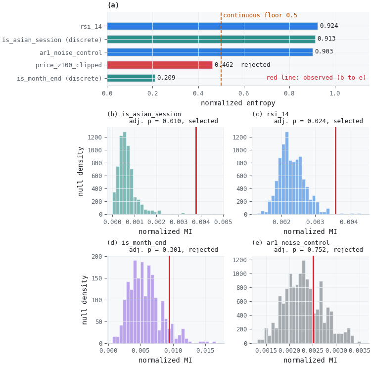
Figure 3. 5-panel illustration of gate 2 entropy and gate 3 mutual-information outcomes on EURUSD H1

• Panel (a): normalized entropy of the five gate 1 survivors; discrete features (teal) are measured at their natural cardinality, continuous features (blue) must clear the 0.5 floor, and the clipped price z-score (red) does not.
• Panel (b): is_asian_session: observed statistic far in the right tail of its null.
• Panel (c): rsi_14: observed statistic in the right tail of its null.
• Panel (d): is_month_end: observed statistic inside the upper part of a wide null.
• Panel (e): ar1_noise_control: observed statistic inside the bulk of its null.

Feature	Observed MI	Null mean	Adjusted p
is_asian_session	0.00377	0.00067	0.010
rsi_14	0.00361	0.00231	0.024
is_month_end	0.00943	0.00569	0.301
ar1_noise_control	0.00251	0.00231	0.753

ScreeningReport(2/9 selected, 4 tested at gate 3, effective_tests=4.0), with scheme="circular_shift", n_perm=500, seed=0. Two features are selected, is_asian_session and rsi_14, the indicator this catalogue already dedicated a full article to in Meta-Labeling the Classics, Part 1. Two features reach Gate 3 and are not selected. is_month_end passed the entropy gate on its level count and has a wide null, and its observed statistic does not stand out from it. ar1_noise_control is the true negative. It reports almost the same entropy as rsi_14 (0.903 against 0.924) and is indistinguishable from it to an entropy-only screen, but its observed value (0.00251) sits inside the bulk of its null (mean 0.00231), and its adjusted p-value of 0.753 says so. Panels (c) and (e) of Figure 3 draw that contrast directly. The effective test count of 4.0 says the four survivors behave like four independent tests, so a worst-case correction would have lost little here.

Three checks bound how far to trust those numbers. First, with 500 resamples the adjusted p-values carry Monte Carlo errors of about 0.005 to 0.02. Repeating the screen with ten seeds keeps both selected features below 0.05 every time (adjusted p between 0.002 and 0.026 for is_asian_session, and between 0.002 and 0.034 for rsi_14), and keeps the two rejected features between 0.23 and 0.80. Second, the calendar-aware null (period=24) keeps both selected, at 0.026 for is_asian_session and 0.002 for rsi_14. Third, switching the Miller-Madow correction off moves raw p-values by less than 0.02 (0.080 against 0.088 for is_month_end, 0.273 against 0.291 for ar1_noise_control) and changes no decision.

The choice of maximum-statistic or minimum-p-value form changes the answer on this family. On the same resamples, westfall_young_maxt gives rsi_14 an adjusted p-value of 0.79 and is_asian_session 0.77, against 0.024 and 0.010 for westfall_young_minp. is_month_end has by far the widest null, so it supplies the family maximum in most replicates and no other feature can beat it. Adding price_level to a family with rsi_14 and ar1_noise_control is worse: its null mean is 0.0167, about seven times that of rsi_14, and rsi_14's maxT adjusted p-value rises to 1.0, while minP gives 0.020.

What kind of information

Mutual information detects dependence of any kind, so a selection is not a claim about direction. Both selected features carry information about the magnitude of the forward return and none that the screen can detect about its sign. For is_asian_session, mutual information against the absolute target is 0.0036 against a null mean of 0.0006 (p = 0.003), while against the sign of the target the p-value is 0.18. The standard deviation of the twenty-bar return is 0.00434 in Asian-session bars and 0.00392 elsewhere, about 11% higher. For rsi_14 the corresponding p-values are 0.010 against the absolute target and 0.27 against the sign. The screen found that both columns tell the model something about how far price will move. It did not find that either tells the model which way.

What the Result Does Not Show

The result is one dataset, one market, and one family of horizons. Several limits follow, and each one bears on how the output should be used.

• The result is horizon-specific. Re-running the same nine columns against a five-bar target selects only is_month_end (adjusted p = 0.002), with rsi_14 at 0.79. Against a sixty-bar target nothing is selected, and rsi_14 is at 0.31.
• Significance is not economic value. Nothing in the screen estimates transaction costs, capacity, or stability out of sample. A feature that clears Gate 3 has information distinguishable from the estimator's noise floor, and no more.
• The false negatives are not counted. A stationary feature lost to a KPSS false rejection, or a rare flag lost to the level-count floor, is not tracked by any correction. The filters cannot create false selections if they never see the target, but they do remove candidates.
• The entropy gate was revised after seeing results. The discrete-feature rule and the quantile-clipped grid were added after an earlier version of this screen rejected both session dummies. The thresholds used here were fixed before the Gate 3 runs reported above, but that revision was informed by earlier output, so the p-values are not free of that history.
• One synthetic control is one true negative. It shows that the screen can reject a persistent null feature. It does not estimate the false-selection rate over many such features.
• The calibration study covers one design. The size results are for a synthetic AR(1) feature, one target, 5,000 bars, and one statistic. Other features, label schemes, or statistics need their own measurement, and part23_size_study.py in the attached files is the template.

Conclusion

Two of nine EURUSD candidates survive, and the count is not the point. Each rejection came with a specific, checkable reason attached: a unit root, a joint-test conflict that an ADF-only gate would have passed, an entropy floor missed by a saturated feature, or a mutual-information statistic indistinguishable from its own null. Each selection came with a null mean, an adjusted p-value, and a measured Monte Carlo error. A screen that reports only "rejected" without the gate and the statistic behind it is not more trustworthy than no screen at all.

Key takeaways:

• Do not screen a persistent feature against an overlapping target with naive_shuffle. The measured false-positive rate was 100% for mutual information and 58% for absolute correlation. Use circular_shift, and add period when either series has a calendar pattern.
• Report the scheme parameters with the result. A stationary bootstrap's size depends on the block length, and every p-value depends on the scheme that generated its null.
• Treat a Gate 1 rejection as routing, not deletion. Transform the feature, re-screen it, and check whether the information survived the transform.
• Set thresholds before looking, not after. Retuning min_entropy after seeing which features it eliminates moves the goalposts on every p-value downstream.
• A selection is a triage result, not a trading signal. Both selected features carry information about the size of the move, not its direction, and neither has been tested for cost or capacity.

Part 24 takes the sequence-risk question this article does not address: even a feature set that clears every gate here can back a strategy whose realized backtest history understates its true drawdown risk, because maximum drawdown depends on the order trades arrived in, and that order is not a property of the strategy.

Revision note. An earlier version of this article reported false-positive rates of 55.5% for naive_shuffle and 6.0% for the other two schemes without naming the test statistic, and described the stationarity and entropy gates as hypothesis-free. The rates in Section 2 were re-measured with the statistic Gate 3 actually uses. Under absolute correlation the re-measured values (58.0%, 3.5%, 4.5%) are close to the earlier ones, and under mutual information they are 100%, 4.1%, and 9.3% at L = 100. The earlier text also said three features fail Gate 1 where four do, and one feature reaches Gate 3 where two do. Gate outcomes, the entropy gate's treatment of discrete features, and the selected set changed as a result of the corrections described above.

Attached Files

	File	Module	Description
1.	permutation.py	afml.screening	Null-generation schemes: naive_shuffle_indices, circular_shift_indices (with period), stationary_bootstrap_indices, resample_indices, bar_permutation, build_null, suggested_block_length.
2.	stationarity.py	afml.screening	Gate 1. assess_stationarity, rolling_stationarity, rolling_power_baseline, stationarity_gate.
3.	entropy_features.py	afml.screening	Gate 2. bin_counts, indicator_entropy, modal_occupancy, entropy_screen.
4.	mutual_information.py	afml.screening	Gate 3. miller_madow_bias, normalized_mutual_info, mi_screen.
5.	multiple_testing.py	afml.screening	Bonferroni, Holm-Bonferroni, Benjamini-Hochberg, Benjamini-Yekutieli, westfall_young_maxt, westfall_young_minp, null_pvalue_matrix, monte_carlo_se, effective_number_of_tests.
6.	pipeline.py	afml.screening	Orchestration. ScreeningReport, screen_features.
7.	report.py	afml.screening	ScreeningResult dataclass binding every statistic to its calibrating null; results_to_frame.
8.	__init__.py	afml.screening	Public exports of the subpackage.
9.	size_calibration.py	afml.screening.notes	Synthetic size study for the resampling schemes.
10.	part23_data.py	afml.screening.notes	EURUSD H1 feature and target construction for this article.
11.	EURUSD_H1_time_2018-01-01-2024-12-31.parq	afml.screening.notes	EURUSD H1 bars, 2018 through 2024 (42,584 aligned bars after feature construction). Keep it in the same folder as part23_data.py.
12.	part23_size_study.py	afml.screening.notes	Size study on the real EURUSD target: schemes, block lengths, persistence, overlap, window length.
13.	part23_screen_demo.py	afml.screening.notes	Full screening run, seed sensitivity, calendar-aware null, minP against maxT, volatility re-screen, horizon check.
14.	test_screening_gates.py	afml.tests	Tests for the three gates and the corrections.
15.	test_screening_permutation.py	afml.tests	Tests for the resampling schemes and result container.
16.	test_screening_revisions.py	afml.tests	Tests for period-restricted rotation, the block-length guard, the conflicting verdict, the power baseline, discrete features, and minP.

Further Reading

• Lopez de Prado, M. (2018). Advances in Financial Machine Learning. John Wiley & Sons.
• Masters, T. (2020). Permutation and Randomization Tests for Trading System Development.
• Masters, T. (2019). Statistically Sound Indicators for Financial Market Trading.
• Politis, D. N., & Romano, J. P. (1994). The stationary bootstrap. Journal of the American Statistical Association, 89(428), 1303–1313.
• Dickey, D. A., & Fuller, W. A. (1979). Distribution of the estimators for autoregressive time series with a unit root. Journal of the American Statistical Association, 74(366a), 427–431.
• Kwiatkowski, D., Phillips, P. C. B., Schmidt, P., & Shin, Y. (1992). Testing the null hypothesis of stationarity against the alternative of a unit root. Journal of Econometrics, 54(1–3), 159–178.
• Hobijn, B., Franses, P. H., & Ooms, M. (1998). Generalizations of the KPSS-test for stationarity. Econometric Institute Report 9802/A.
• Schwert, G. W. (1989). Tests for unit roots: a Monte Carlo investigation. Journal of Business & Economic Statistics, 7(2), 147–159.
• Westfall, P. H., & Young, S. S. (1993). Resampling-Based Multiple Testing. John Wiley & Sons.
• Bourgon, R., Gentleman, R., & Huber, W. (2010). Independent filtering increases detection power for high-throughput experiments. Proceedings of the National Academy of Sciences, 107(21), 9546–9551.
• Miller, G. A. (1955). Note on the bias of information estimates. Information Theory in Psychology: Problems and Methods, 95–100.
• Cover, T. M., & Thomas, J. A. (2006). Elements of Information Theory (2nd ed.). John Wiley & Sons.