MetaTrader 5 Machine Learning Blueprint (Part 22): Auditing the Selection Criterion — Measuring Overfit in Hyperparameter Search

Table of Contents

1. Introduction
2. What Nested CV Fixed, and What It Left Alone
3. Bias and Variance in Model Selection
4. Making the Criterion's Variance Measurable
5. Auditing the Criterion (criterion_variance_audit)
6. The Selection Optimism Curve
7. Every Knob Is an ARD Length-Scale
8. Three Remedies, and a Bug in the One We Already Had
9. Hyperparameter Trials Are Backtest Trials
10. The Median Protocol, and Where It Is Actually Fine
11. Running the Audit on Your Own Bars
12. Conclusion
13. Attached Files
14. References

Introduction

In Part 16 we moved hyperparameter search inside every outer fold and reported the resulting nested score instead of the search's own best value. That closed a specific hole: the number we publish is now an estimate of what the pipeline does on data it has never touched, rather than the maximum of a quantity the search spent hundreds of trials maximizing.

It closed one hole and left a larger one open. Nested cross-validation makes the reported figure honest about the damage; it does not reduce the damage, and — importantly — it does not isolate the damage attributable to selection overfitting specifically. Nested CV evaluates the entire pipeline end-to-end. If the reported score is poor, the cause could be selection overfitting, a regime shift between folds, label noise, an unstable feature set, or any combination of them. To attribute the shortfall to selection overfitting alone, a counterfactual benchmark is needed: an oracle that knows the best hyperparameters, or a fixed-hyperparameter pipeline scored on the same folds, or an independent resampling of the selection procedure. This article builds the diagnostic tools, but the reader should be clear from the start that the resolution ratio below measures the local discriminating power of the criterion, not the total damage of the pipeline. Those are related but distinct quantities. The search still tunes hyperparameters against a finite sample, still finds whatever peculiarities that sample contains, and still hands back a model shaped partly by noise. Nothing in the pipeline asks the prior question: on this sample, with this criterion, is the search capable of distinguishing one hyperparameter vector from another at all?

This article answers that question with a number. We implement afml.cross_validation.selection_overfit. It measures the criterion's dispersion across legitimate repartitions of the same data, compares it with the dispersion across candidates, and reports their ratio — specifically, the ratio of candidate spread to noise floor (signal-to-noise, not noise-to-signal). In the study below the ratio is 0.49. The criterion's noise is about twice the spread it is expected to resolve. Under that condition the search selected the candidate that is best on average on one partition in eight, and on this particular sample its held-out score was beaten by twenty-six of the sixty candidates it rejected. (As Section 6 explains, that last number does not by itself prove that uniform random selection would have done better; it shows only that the specific candidate chosen by the argmax was not the one that generalized best.)

Three consequences follow, and each gets a section. Under a fixed trial budget on this simulated data, widening the search space improved the reported criterion and degraded the deployed model. That is a specific instance of Cawley and Talbot's ARD result, not a universal law: given enough budget, enough signal, or enough regularization, a wider space can win. The remedy is not a better sampler but a lower-variance criterion, which changes how early stopping should be thresholded. And because a Bayesian sampler produces correlated trials, the trial count that belongs in the Deflated Sharpe Ratio is neither the raw number of Optuna trials nor the one we currently pass.

The reference throughout is Gavin Cawley and Nicola Talbot's On Over-fitting in Model Selection and Subsequent Selection Bias in Performance Evaluation (JMLR, 2010). Part 16 implemented their Section 5. This article implements their Section 4, which is the part that tells you what to do differently. Their experiments are on stationary UCI benchmarks with i.i.d. folds. Transferring the conclusions to financial data requires additional assumptions — stationary enough features, a loss with bounded influence, dependence handled explicitly, and a search algorithm whose exploration matches the space — which we flag at each relevant step.

What Nested CV Fixed, and What It Left Alone

Cawley and Talbot separate two failures that are easy to conflate.

The first is selection bias in performance evaluation. If hyperparameters are chosen using data that later appears in the evaluation set, the evaluation is optimistic, because the hyperparameters retain a partial memory of that data. The fix is structural: perform model selection afresh inside every resampling of the data, so that no observation ever informs the settings under which it is scored. That is nested cross-validation, and that is Part 16.

The second is overfitting in model selection itself. The search minimizes a criterion evaluated on a finite sample. Beyond some point, further minimization no longer improves generalization; it exploits features of that particular sample. Cawley and Talbot show the classic training-overfit signature reproduced one level up, with the criterion falling monotonically while the true error turns and climbs after roughly thirty to forty optimization steps.

Nested CV addresses the first and is largely silent on the second. It does not isolate the second from other sources of held-out degradation: regime drift, label noise, feature instability, and sampling variation all contribute to a poor nested score, and nested CV reports only their sum. Running the search inside each outer fold does not make the search better; it makes each fold's search independently overfit and then averages the resulting damage into an honest number. If the criterion has high variance, the nested score will be honestly poor, and the pipeline will offer no diagnosis and no lever.

The distinction matters operationally because the two problems call for opposite responses. Selection bias is fixed by adding structure and compute. Overfitting in model selection is usually fixed by searching less: fewer hyperparameters, fewer trials, a lower-variance criterion, and a selection rule that declines to distinguish candidates the data cannot separate.

Bias and Variance in Model Selection

Let G(θ) be the true generalization performance of a model with hyperparameters θ, and g(θ;D) an estimate computed on a finite sample D. The expected squared error of the estimator splits into a squared bias term and a variance term in the usual way.

For performance evaluation, bias is what matters: we want the reported number to be right on average. For model selection, it is not. Selection never uses the level of the criterion, only its shape: all we need is for the minimizer of g to sit near the minimizer of G. A criterion that is uniformly pessimistic by a constant is a perfect selection criterion, because a constant offset moves no minimum. A criterion that is unbiased but noisy is a poor one, because its minimum lands in a different place on every sample.

This is the inversion that makes leave-one-out cross-validation a worse selection criterion than its unbiasedness suggests, and it is the reason a five-fold estimate scored on a small validation block can be actively misleading no matter how carefully it is purged.

Bias and variance of the selection criterion

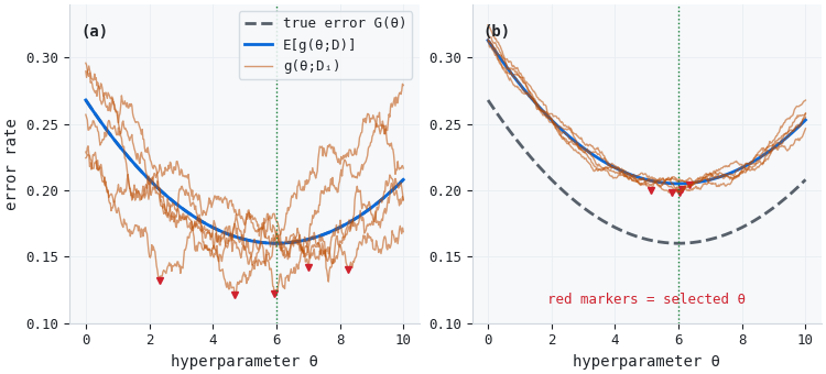
Figure 1. Two-panel illustration of why variance dominates bias in model selection

• Panel (a): an unbiased criterion whose expected value sits exactly on the true error curve. Individual sample realizations swing widely, and the selected θ lands far from the true optimum on most draws.
• Panel (b): a criterion biased upward by a constant. Every realization is wrong about the level and nearly right about the location, so the selected θ clusters tightly on the true optimum.

The criterion in panel (b) would be rejected by any test of unbiasedness and is the better tool for the job. That is the whole argument, and everything that follows is an attempt to measure which panel a given pipeline is in.

Making the Criterion's Variance Measurable

There is an obstacle. PurgedKFold partitions the sample deterministically: the test blocks are contiguous positional slices, so the same data always yields the same folds and the same score. One number has no dispersion. The quantity we need to measure is invisible by construction.

Shuffling is not available to us. The folds are contiguous precisely because the labels overlap in time and the embargo has to mean something. What is available is a boundary shift. Advancing the first test block by a few samples produces a different partition of the same series that is equally legitimate: blocks stay contiguous, order is preserved, and purging and embargo apply exactly as before. Evaluating one fixed θ across several offsets gives several draws of the criterion, and their standard deviation is an estimate of the noise floor.

A caveat that the diagnostic relies on but does not eliminate: the offsets are not independent draws. Adjacent offsets produce partitions that share most of their observations and most of their folds; the correlation between draws can be high. The standard deviation across offsets therefore estimates the dispersion of the criterion under a particular family of dependent repartitions, and it can be biased in either direction relative to the true sampling variability of the criterion under an independent draw of comparable data. Read it as a lower-bound estimate of the criterion's variance when in doubt: an audit that reports a low resolution ratio is still informative, but one that reports a high resolution ratio should not be treated as proof that the search is safe.

One purged fold under three boundary offsets

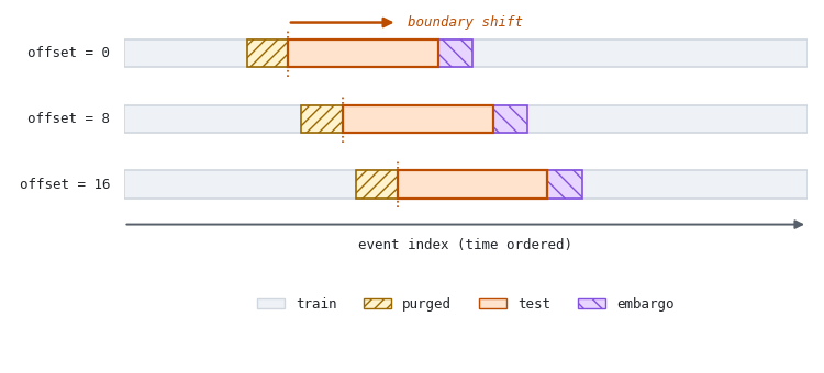
Figure 2. Three-row illustration of the boundary shift that generates repartitions

• Row 1: the standard partition, offset zero. The test block opens at a fixed position and the purge region precedes it.
• Row 2: the same fold advanced by eight events. The purge and embargo regions travel with the block.
• Row 3: advanced by sixteen. Every row is a valid purged, embargoed split of the same series, so the three criterion values are three correlated draws of the same quantity.

OffsetPurgedKFold implements this. It is a drop-in for PurgedKFold with one extra argument, and offset=0 reproduces the standard partition.

class OffsetPurgedKFold(BaseCrossValidator):
    """Purged, embargoed K-fold whose test blocks start at an arbitrary offset."""

    def split(self, X, y=None, groups=None):
        if not X.index.equals(self.t1.index):
            raise ValueError("X.index and t1.index must be identical")

        n        = X.shape[0]
        indices  = np.arange(n)
        embargo  = int(n * self.pct_embargo)
        t1_vals  = self.t1.values
        t1_idx   = self.t1.index.values

        for start, stop in self._test_blocks(n):
            test_idx = indices[start:stop]
            test_t0  = t1_idx[start]
            test_t1  = t1_vals[test_idx].max()

            # Left block: events that closed strictly before the test opened.
            left = indices[t1_vals < test_t0]
            left = left[left < start]

            # Right block: events starting strictly after the last test label
            # closed, plus the embargo.
            right_start = int(np.searchsorted(t1_idx, test_t1, side="right"))
            right_start = min(right_start + embargo, n)

            train_idx = np.concatenate([left, indices[right_start:]]).astype(int)
            if train_idx.size == 0 or test_idx.size == 0:
                continue
            yield train_idx, test_idx

Two boundary conditions are strict here where AFML Snippet 7.1 is loose. A label closing exactly on the first test timestamp overlaps the test window under the snippet's own inclusive overlap definition, and the original PurgedKFold keeps it via t1 <= t0. We drop it. Likewise searchsorted is called with side="right" so that an event starting exactly when the last test label closes is excluded rather than admitted on a zero embargo. Both changes are one-sample effects that a test for leakage will catch and a backtest will not. If your event convention treats the label interval as half-open, [t0, t1), the strict exclusions here are one observation too conservative. The default is the inclusive convention because AFML uses it; adjust if your pipeline does not.

A note on nesting purged folds: do not feed a PurgedKFold outer training set directly into another PurgedKFold. The outer training set is not contiguous: it is a left block, a gap, and a right block. The inner splitter will carve contiguous positional slices across that concatenation, so an inner test block can straddle the gap, and the embargo, computed as a fraction of the row count rather than as a span of time, will silently embargo the wrong observations on the far side of the discontinuity. This is a statement about splitting on positional concatenated indices. If the inner splitter operates on the original timestamps and applies purge logic against the same time axis, the objection does not apply and nesting is perfectly legitimate. Part 16 avoids the concatenation problem by running the inner loop with PurgedWalkForwardCV over a contiguous training block.

Auditing the Criterion (criterion_variance_audit)

With repartitioning available, the audit is direct. Score every candidate on every offset. The dispersion of one candidate's score across offsets is the noise; the dispersion of candidate means is the signal. Their ratio decides whether the search is estimation or noise mining.

report = criterion_variance_audit(
    estimator, X, y, t1, param_candidates=grid,
    sample_weight=sw, n_splits=5, pct_embargo=0.01,
    n_resamples=10, scorer=neg_log_loss_scorer,
)
print(report.summary())

Four quantities come back. The noise_floor is the mean across candidates of the criterion's standard deviation over partitions. The candidate_spread is the standard deviation across candidates of the partition-averaged score. The resolution_ratio is defined as candidate_spread / noise_floor — signal divided by noise. A value above one means the criterion can discriminate candidates by more than its own dispersion; below one the search cannot separate candidates from sampling noise. The selection_regret is the expected shortfall, in criterion units, between what the argmax on a single partition delivers and what the candidate that is best on average delivers, with argmax_stability reporting how often those coincide.

Two clarifications on what these numbers mean. First, selection_regret is not an out-of-sample regret in the backtest sense. It measures the shortfall on the same repartitions used to define the surrogate "truth" (the partition-averaged score). It is an internal quantity. A true out-of-sample regret would require scoring the selected and best-on-average candidates on an independent future period, which the audit does not do. Second, argmax_stability measures agreement with the partition-averaged best, not correctness in any absolute sense. A candidate can be stable under this metric and still be far from the true optimum of G.

One further caveat: candidate_spread is a property of the candidate set, not of the criterion. Adding obviously bad candidates to the grid inflates the spread without improving the search's ability to distinguish the leaders. The number that matters for selection is the local distinguishability of the top few candidates, not the overall spread across the entire grid. Read the resolution ratio together with the per-candidate table, and prefer interpretations that look at the top of the ranking rather than at the extremes.

The study below uses a simulated market with four thousand hourly bars and GARCH cluster volatility. It includes a slowly switching latent state that flips the sign of a weak momentum term. We use twelve features (two signal, ten noise) and overlapping forward-return labels thinned to one thousand events (base rate 0.503). The simulation is not a claim about any instrument. It is a controlled instance of the regime that matters, in which a small unstable edge sits under mostly-noise features and the labels overlap. Section 11 covers running the same audit on real bars, which is where the number you should act on comes from.

Criterion variance and the instability it produces

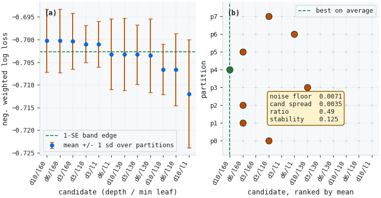
Figure 3. Two-panel illustration of a selection criterion that cannot resolve its candidates

• Panel (a): twelve candidates ranked by mean score, with error bars spanning one standard deviation over the eight partitions. The bars overlap almost completely; the dashed line is the one-standard-error band edge, and five candidates fall inside it.
• Panel (b): the argmax on each partition. The dashed line marks the candidate that is best on average, and only partition p4 selects it. The winner moves across five distinct candidates as the fold boundary shifts.

Quantity	Value	Reading
Criterion noise floor	0.00710	Dispersion at fixed θ
Candidate spread	0.00350	Dispersion across θ
Resolution ratio	0.49	Below one: noise dominates
Selection regret	0.00093	Internal cost of trusting the argmax
Argmax stability	0.125	Matches partition-averaged best on one in eight

The noise floor is twice the candidate spread. The ranking in panel (a) is therefore mostly an artifact of where the fold boundaries happened to fall, and panel (b) shows exactly that: shift the boundary and a different candidate wins. Reporting the argmax as "the tuned model" describes a coin flip in the language of optimization.

The resolution ratio is the one number worth carrying forward. The operational thresholds below are heuristic, not derived. They are not read off an error model or a confidence interval, and they will need recalibration on each dataset. Treat them as a starting vocabulary, not a decision rule with a p-value:

• Above roughly two, the search is likely doing estimation and its output can be used as a guide. Even here, prefer a tolerance band to a hard argmax.
• Between one and two, treat the ranking as approximate and prefer a selection rule with a tolerance band.
• Below one, the argmax carries little information the data supports. This does not mean the ranking is useless: extreme candidates can still be distinguished reliably, and a reduced candidate set is often sufficient. But the specific top-1 selection is unlikely to be reproducible, and the honest options are to widen the criterion's evidence base, reduce the candidate set, or stop distinguishing leaders altogether.

The Selection Optimism Curve

The audit measures the criterion at a fixed set of candidates. The complementary view tracks what happens as a search consumes its budget. selection_optimism_curve cuts the sample once in time order, purges the boundary, then for each trial scores a sampled θ by purged CV inside the design set, refits on the whole design set, and scores the refit on the held-out block. The incumbent is whichever trial leads on the inner criterion.

One split is one observation. The numbers below — correlation, optimism gap, number of rejections beating the selection — are estimates from a single time anchor. On real data with regime drift, the sign of the correlation can depend on the split position. A negative correlation observed once is suggestive; a negative correlation reproduced across several time anchors, or across several instruments, is evidence. Section 11 states this as a reproduction requirement for a reason.

curve, fold_scores = selection_optimism_curve(
    estimator, X, y, t1, param_sampler,
    n_trials=60, sample_weight=sw,
    design_fraction=0.70, n_splits=4, n_offsets=3,
    scorer=neg_log_loss_scorer, random_state=11,
    return_fold_scores=True,
)

Inner criterion against held-out performance across the search

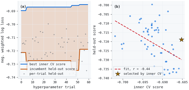
Figure 4. Two-panel illustration of selection optimism over a sixty-trial search

• Panel (a): the best inner score climbs in steps as the incumbent changes, while the incumbent's held-out score moves independently and mostly downward. The shaded region between them is the optimism gap.
• Panel (b): every trial plotted as inner score against held-out score, with the fitted slope and the star marking the trial the search selected. The relationship is negative.

The gap runs between 0.034 and 0.049 nats, around five percent of the log-loss level, and it does not close with more trials. The more interesting number is in panel (b): across the sixty trials the correlation between the inner criterion and held-out performance is −0.44. On this sample, the criterion was not merely noisy — it was anti-informative, and on this split the model selected by the argmax had a worse held-out score than twenty-six of the sixty candidates it rejected.

What that number does and does not establish. Twenty-six of sixty rejected candidates beat the selected one. That does not imply uniform random selection would have done better; 33 of 60 did not beat it, and the average held-out score of all candidates would need to be compared against the selected candidate's score to make that claim. What the observation supports is narrower: the argmax on the inner criterion is not a reliable proxy for held-out performance on this sample. That is enough to justify the remedies below, and it does not require overclaiming.

The mechanism is straightforward and should be stated plainly. The simulator embeds a slowly switching latent regime, and the held-out block sits after the design block in time. A model that fits the design-period regime harder scores better inside it and worse afterward. That is a property of markets, not an artifact introduced to produce a striking figure, and it is why the sign can invert on price data in a way it rarely does on the stationary UCI benchmarks Cawley and Talbot used. But the confounding must be stated: on this simulation, the negative inner/held-out correlation is at least partly driven by the regime shift, not by selection overfitting alone. The regime shift depresses the inner/held-out correlation independently of any selection effect. The audit cannot, in this design, decompose the two. On real data with unknown regime structure, the same caution applies: a negative correlation is evidence of something, not necessarily of selection overfitting specifically. The robust claim is the resolution ratio below one, of which the instability of the argmax is a consequence; whether the inner/held-out correlation inverts is a question the diagnostic cannot answer in isolation.

Every Knob Is an ARD Length-Scale

Cawley and Talbot's most useful empirical result compares two kernels. An ARD kernel gives every input dimension its own length-scale; an isotropic RBF kernel shares one across all of them. ARD nests RBF, so the best test error achievable with ARD can never be worse. On twelve of thirteen benchmarks, RBF won anyway, and the PRESS statistic was lower for ARD on most of them. More knobs produced a better criterion and a worse model.

The transposition to Optuna is suggestive but not exact. An ARD length-scale is a model parameter in a specific kernel, with a smooth likelihood landscape and clear gradient structure. A hyperparameter in an Optuna space can be a regularization strength, a sampling parameter, a compute budget, or a stochastic parameter, and different knobs interact differently with the criterion. The analogy holds because each added dimension is a way for the search to fit criterion noise, but the specific dynamics — how the optimum moves as the space widens, how the trial budget interacts with the dimensionality — are not the same. The empirical result below should be read as a demonstration that the ARD finding can reproduce on financial-style data, not as a proof that it always will.

There is a second caveat that is important because it is easy to get wrong. ARD nests RBF, so with an ideal optimizer and an unbounded trial budget the wider space cannot do worse. With a fixed budget, that nesting guarantee does not hold. Forty trials on a six-dimensional space may not visit the region corresponding to the two-dimensional subspace at all. The wider space can lose not only because it overfits, but because the sampler's coverage is thinner. Both effects push in the same direction here, and the diagnostic below does not separate them.

We ran it. Same estimator, same data, same forty-trial budget, same partitions, same seed. The narrow space searches two parameters that control the bias-variance trade-off directly, max_depth and min_weight_fraction_leaf, with everything else fixed. The wide space adds min_samples_leaf, max_features, n_estimators and max_samples, and contains the narrow space as a subset.

Search-space width against generalization

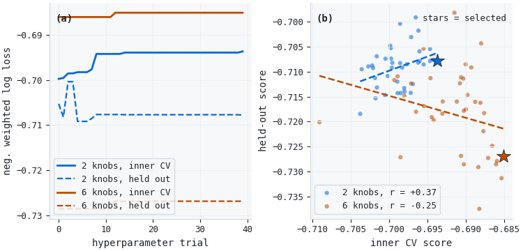
Figure 5. Two-panel illustration of the ARD result transposed to a hyperparameter space

• Panel (a): incumbent trajectories for both spaces. The wide space holds the highest inner score and the lowest held-out score simultaneously; the two orange lines bracket both blue ones.
• Panel (b): inner against held-out score for all forty trials in each space, with fitted slopes. The narrow space keeps a positive relationship; the wide space inverts it.

Quantity	Narrow, 2 knobs	Wide, 6 knobs
Best inner score	−0.6937	−0.6851
Held-out score	−0.7078	−0.7269
Optimism gap	0.0141	0.0417
corr(inner, held out)	+0.37	−0.25
Trials beating the selection	13 of 40	29 of 40

The wide space wins the criterion by 0.0086 nats and loses out of sample by 0.0191 on this setup, at this budget, on this data. The optimism gap triples. The correlation flips sign. This is Table 2 of the paper reproduced on price-style data under conditions favourable to the effect: a small sample, a fixed trial budget, and a latent regime shift. It is not a general law that wider spaces always lose. Given a much larger budget, a smoother criterion, or a search space whose extra dimensions are genuinely irrelevant (in which case a good sampler will quickly learn to ignore them), a wider space can and does win. The design rule that follows is not "never widen" but "widen deliberately, and expect the extra dimensions to cost you something at typical budgets."

The design rule that follows is to search only the parameters that control model capacity directly and to fix the rest by argument. For a Random Forest, max_depth and min_weight_fraction_leaf control capacity; n_estimators is a compute budget with a monotone and saturating effect and does not belong in a search at all; max_features and min_samples_leaf have second-order effects that the criterion above cannot resolve anyway. Fixing them is the isotropic-kernel choice: theoretical flexibility traded for a criterion whose minimum means something.

Three Remedies, and a Bug in the One We Already Had

Cawley and Talbot note that the remedies for overfitting in model selection are the remedies for overfitting in training: regularization, early stopping, and averaging. All three are implemented here, and the first was already in the codebase with two defects.

Regularization: the one-standard-error rule, corrected

Selecting the simplest candidate within one standard error of the best is a variance-reduction device: it declines to distinguish candidates the data cannot separate. The implementation in inner_cv_search got two things wrong.

The first is arithmetic. The tolerance was computed as np.std(fold_scores), the standard deviation of the fold scores, where the rule calls for the standard error of the fold mean, std / sqrt(k). On nine folds the band is three times too wide. What is meant to admit statistically indistinguishable candidates instead admits candidates that are genuinely worse, and since the selection then takes the simplest of them, the rule degenerates into an unconditional preference for the smallest model in the grid. It was not regularizing; it was under-fitting on purpose, silently.

The second is the definition of "simplest". The code took within_1se[0], relying on ParameterGrid ordering to run from coarse to fine. It does not. ParameterGrid iterates in sorted-key order with the last key varying fastest, which is a property of the dictionary's keys and has nothing to do with model capacity. Rename a parameter and the selection changes. Complexity has to be stated.

A correction that the code comment omits: the std / sqrt(k) divisor assumes the fold scores are independent or weakly dependent. Purged CV removes leakage between training and test, but it does not make the fold scores independent of each other — adjacent folds share overlap structure, share the same underlying regime, and their errors are correlated. The true standard error of the fold mean under positive fold correlation is larger than std / sqrt(k), which means the corrected rule is still somewhat too permissive. It is much closer to correct than the original, and it is the standard adjustment. Readers who want a stricter band should inflate the divisor by a factor estimated from the fold-score correlation matrix, or simply widen the tolerance by hand.

def one_standard_error_selection(results, complexity, score_key="fold_scores",
                                 param_key="params"):
    table = []
    for r in results:
        fs = np.asarray(r[score_key], dtype=float)
        if fs.size < 2:
            raise ValueError("each candidate needs at least two fold scores")
        table.append({
            "entry":      r,
            "mean":       float(fs.mean()),
            "se":         float(fs.std(ddof=1) / np.sqrt(fs.size)),   # not fs.std()
            "complexity": float(complexity(r[param_key])),        # not grid order
        })

    best      = max(table, key=lambda d: d["mean"])
    threshold = best["mean"] - best["se"]
    within    = [d for d in table if d["mean"] >= threshold]
    chosen    = min(within, key=lambda d: d["complexity"])
    return chosen["entry"], {...}

On the audited grid the argmax is depth 10 with a minimum leaf of 60; the corrected rule keeps five of twelve candidates inside a band of 0.00247 and selects depth 3 with the same leaf constraint. Given an argmax stability of 0.125, discarding the ranking within the band is not a concession. It is the only defensible reading of the evidence.

On the complexity callable: the article cannot prescribe how to compare complexity across conditional hyperparameters (e.g., a parameter that only applies when another parameter takes a particular value). Choose a callable that is meaningful for your model, document it, and be aware that a poorly chosen complexity function can silently bias the selection in either direction. For Random Forest, depth and minimum leaf size are sufficient in practice. For pipelines with mutually exclusive branches, define complexity as a tuple comparison and accept that the ordering is a modelling decision, not a fact.

Early stopping, thresholded by the noise floor

Early stopping needs a threshold, and an arbitrary epsilon is the wrong one. The threshold that means something is the dispersion of the criterion itself: an improvement smaller than one standard deviation of the criterion at fixed hyperparameters is not evidence of a better model. HPOEarlyStopping takes the noise floor from the audit and requires improvements to clear it.

This is a heuristic, not a hypothesis test. The difference between the incumbent's score and the challenger's score is a difference of two noisy estimates; its variance is not necessarily equal to the variance of a single fixed-θ score. In particular, the incumbent is a maximum over trials, so its score is biased upward relative to the underlying performance; the difference is not distributed as the noise floor. The threshold used here is deliberately conservative in the direction of stopping early — it treats any improvement smaller than one noise floor as indistinguishable from noise. Under repeated trials, the chance of a spurious "improvement" that clears the noise floor also accumulates, so a stricter threshold is warranted when the budget is large. If you need a genuine test, use a paired comparison on the fold-score vectors or a permutation test on the split boundaries, and adjust for the number of trials.

audit = criterion_variance_audit(estimator, X, y, t1, probe_grid, n_resamples=8)

study.optimize(
    objective,
    n_trials=200,
    callbacks=[HPOEarlyStopping(
        noise_floor=audit.noise_floor,
        patience=15,
        min_trials=20,
        tolerance_multiple=1.0,
    )],
)

Two implementation points are worth flagging because the obvious version fails. Pruned and failed trials carry trial.value is None, so any callback that reduces over recent trial values raises a TypeError the first time a pruner fires, and the codebase already uses MedianPruner. The callback checks for None and returns. And a stopping rule with no tolerance resets its patience counter on an improvement of one part in a billion, which is precisely the failure the noise floor is there to prevent.

Averaging over the leaders

When the resolution ratio is below one, the ranking among the top candidates is noise, so committing to the single argmax spends real capital on a coin flip. top_m_ensemble fits the M best-scoring vectors and averages their predicted probabilities, keeping the region the search identified while discarding the ordering it cannot justify. A reasonable M is the number of candidates inside the one-standard-error band. The cost is M forward passes at inference, or an ONNX graph that averages the members.

Hyperparameter Trials Are Backtest Trials

The Deflated Sharpe Ratio deflates an observed Sharpe by the expected maximum of N trials, and the pipeline gets N from StrategyTrialTracker, which counts manually logged strategy variants. A two-hundred-trial Optuna study currently enters that count as one. Every one of those trials selected a model on the same data, and the winner is a maximum over two hundred draws just as surely as if we had hand-tested two hundred moving-average pairs.

The mapping is a conservative adjustment, not a theorem. A hyperparameter trial is not a separate backtest in the sense the Deflated Sharpe Ratio was formulated for. The DSR assumes N trials whose performance metrics are Sharpe ratios with a known variance; here we have N trials whose selection criterion is log loss on cross-validation folds, and the relationship between a fold-score vector and a Sharpe distribution is indirect. Treating HPO trials as backtest trials is a precaution against under-deflation, and it errs on the side of rejecting strategies. That is the correct error direction for deployment. It is not a rigorous consequence of the DSR definition, and readers who need a formally justified count should construct it from the trial PnL distributions themselves rather than from fold scores.

Passing the raw trial count is also wrong, but in the opposite direction. A TPE sampler concentrates draws in a region of the space, so successive trials make nearly the same errors on nearly the same observations, and the expected maximum of two hundred strongly correlated trials is far below that of two hundred independent ones.

effective_trial_count takes the per-trial score vectors and returns two standard estimates: the eigenvalue estimator of Li and Ji (2005), summing the integer and fractional parts of the eigenvalues of the trial correlation matrix, and the Kish (1965) design effect under equicorrelation.

Trial redundancy and the Sharpe hurdle it implies

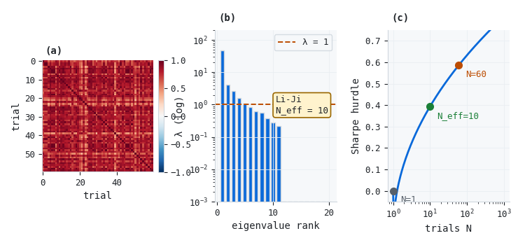
Figure 6. Three-panel illustration of correlated trials and the deflation they require

• Panel (a): the correlation matrix of the sixty trials' fold-score vectors, uniformly dark. The mean pairwise correlation is 0.787.
• Panel (b): the eigenvalue spectrum. One component of magnitude 47 dominates and the remainder sit near the unit line, so the sixty trials explore close to one direction.
• Panel (c): the expected maximum Sharpe against trial count, with markers at N equal to one, the effective count, and the raw count.

Trial count used	Value	Sharpe hurdle
Current pipeline (HPO uncounted)	1	0.00
Effective, eigenvalue estimator	10.0	0.39
Effective, Kish design effect	1.26	0.06
Raw trial count	60	0.59

The practical finding is the first row against the last: leaving hyperparameter trials out of the deflation understates the Sharpe hurdle by roughly 0.4 to 0.6 on this study. A strategy reporting a backtested Sharpe of 0.5 clears a hurdle of zero and fails against both effective counts.

The two estimators disagree by an order of magnitude here, and the reason is stated by the function rather than hidden. Here the correlation matrix is built from sixty vectors of length twelve, so its rank is at most eleven. As a result, the eigenvalue estimator cannot report much more than ~12 effective trials, regardless of how many were run. The result is flagged rank_limited and should be read as a floor. The fix is to lengthen each trial's score vector by scoring across several fold-boundary offsets, which is what the n_offsets argument to selection_optimism_curve is for; with sixty trials, aim for a vector length above sixty before trusting the estimate.

When the estimate is rank-limited, the correct fallback depends on which direction of error you can tolerate. The raw count is a conservative upper bound: it over-deflates, which can reject a genuinely good strategy. The eigenvalue estimate is a floor: it under-deflates, which can admit a genuinely bad one. For deployment decisions, prefer the conservative direction and use the raw count. For research decisions — understanding what your search actually explored — the effective estimate is more informative even when rank-limited, provided you read it as a lower bound rather than a point estimate.

The Median Protocol, and Where It Is Actually Fine

Cawley and Talbot devote their Section 5.2 to a protocol that tunes hyperparameters on the first few folds, takes the median, and then scores every fold with those frozen values. It is optimistically biased on eleven of thirteen benchmarks, the bias exceeds the typical difference between competing classifiers on four of them, and it is biased by different amounts for different algorithms, so it does not even rank methods correctly. Their conclusion is that it should be deprecated.

Three evaluation protocols and their trading analogues

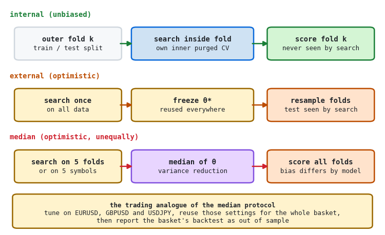
Figure 7. Three-row illustration of internal, external and median evaluation protocols

• Row 1: the internal protocol. Each outer fold runs its own inner purged search, and the fold is scored by a model that never saw it. This is Part 16.
• Row 2: the external protocol. One search over all data, frozen settings, then resampled folds whose test data informed those settings.
• Row 3: the median protocol. Search on a few folds, take the median, score everything. Adds variance reduction on top of the external bias.
• Callout: the version that appears in trading work, where the folds are symbols rather than time blocks.

The trading form is worth naming because it does not look like the thing being warned about. Tune on EURUSD, GBPUSD and USDJPY; take the settings that worked across all three; run the whole basket with those settings; report the basket's backtest as out of sample. Every element of the median protocol is present. The three tuning symbols are correlated with the rest of the basket, so their test data is not clean, and taking the consensus across three symbols is a variance-reduction step that flatters the result exactly as the median over folds does.

Here is where the paper's conclusion needs a qualification it does not make, and this is the one point in this article where I would push back on it. The bias Cawley and Talbot demonstrate is a bias in a reported number. Every experiment they run measures a difference between error rates estimated under two protocols. That is an argument against the median protocol as an evaluation procedure and it says nothing about aggregation as a deployment choice.

Once the nested score has been reported honestly, no published figure depends on how the shipped hyperparameters were chosen. At that point aggregating the per-fold winners is a variance-reduction device applied to a decision rather than to an estimate, and it is a reasonable one for the same reason the median protocol flatters results: the median of several noisy selections is usually better than any one of them. But the deployed model is not thereby validated. The nested score is valid for the procedure the nested loop evaluated — a search and fit inside each outer fold. The aggregated-parameter model is a different procedure: it takes medians of per-fold winners and refits on the full sample. Nothing in this article establishes that its performance matches the nested score, and if a performance estimate for the deployed model is going to be reported, it must be estimated separately, from data not used to build it. The claim we can make is narrower: the deployed model's hyperparameters were chosen without contaminating the nested score, provided the sequence below is followed.

The rule is a sequence, not a prohibition. Aggregate after the score is reported, never before, and never re-score with the aggregate.

aggregate_fold_params implements this with the type handling that the obvious version gets wrong. Python's statistics.median of an even-length integer list returns the mean of the two central values, so median([3, 4]) is 3.5 and max_depth=3.5 raises inside scikit-learn — and an even number of outer folds is the common case. Booleans are the second trap: isinstance(True, int) is true in Python, so a naive numeric branch silently averages bootstrap flags. Integer keys are rounded back to integers, booleans resolve by majority, and categorical or None-bearing keys take the modal value.

One limitation the type handling does not solve: conditional hyperparameters. If one key's valid values depend on another key's value — as with a kernel choice that determines whether a gamma parameter applies — taking medians per key independently can produce an invalid combination. The function does not detect this, and no aggregation function can without a schema. Inspect the aggregated parameters before fitting and, if the space contains conditional keys, aggregate per conditional branch instead of across the whole set.

nested_score = report_nested_cv(...)          # publish this, and only this

deploy_params = aggregate_fold_params(        # then choose what to ship
    [fold["best_params"] for fold in outer_results],
    numeric_agg="median",
)
final_model = clone(estimator).set_params(**deploy_params).fit(X_all, y_all, sample_weight=sw_all)
export_onnx(final_model, "EURUSD_H1.onnx")

The alternative to aggregation is the top-M ensemble from the previous section, which sidesteps the choice entirely by refusing to collapse the leaders into one vector. Prefer it when inference cost allows and the band is wide; prefer the aggregate when a single ONNX graph is a hard requirement.

Running the Audit on Your Own Bars

The study above is simulated, and it should be read as establishing a mechanism rather than a fact about any market. This mirrors the structure of the source paper: Cawley and Talbot demonstrate overfitting in model selection on a synthetic benchmark where ground truth is available, then devote a separate section to establishing that it is a genuine concern on real data. The synthetic half is the part that explains; the real half is the part that decides whether to act. The numbers in Figures 3–5 are not transferable as magnitudes. On real data with strong signal, a stable regime, or a well-specified model, the resolution ratio may be well above one, the inner/held-out correlation may be positive, and widening the search space may be entirely justified. Run the audit and let it answer for your data.

The audit needs nothing from the simulation. It needs a feature matrix, binary labels, an event end-time series for purging, and optionally sample weights, all sharing one index. The attached run_real_audit.py takes a bar file and emits the three quantities that matter.

python run_real_audit.py --parquet /data/eurusd_h1.parquet --n-trials 60 --n-resamples 10

Substitute the production feature panel and the triple-barrier events from Part 2 for the stand-in block in that script, and the numbers describe the pipeline actually being shipped rather than an approximation of it. Three questions are worth answering before the next search is run:

1. What is the resolution ratio on the real event set? Below one, the current hyperparameters are a coin flip and the search budget is being spent on nothing.
2. Does the correlation between the inner criterion and held-out performance stay positive, and does it stay positive across several time anchors? A single negative value on real bars is a warning, not proof; a negative value reproduced at several anchors is a much stronger statement. Note also that regime shift and selection overfitting both depress this correlation, and a single-split measurement cannot separate them.
3. How many effective trials has the study accumulated, and does adding that count to the Deflated Sharpe Ratio change any conclusion already drawn?

One caution on scoring. The criterion should be log loss or Brier, not F1 or accuracy. A thresholded metric is discontinuous in the model's parameters and has visibly higher variance than a proper scoring rule on the same folds, which is the wrong property for a quantity whose variance is the subject of the exercise. Choosing a high-variance criterion and then auditing its variance is a way to guarantee the answer.

Conclusion

Part 16 made the reported number honest. This article addresses the process that number describes.

The measurement that drives everything is the resolution ratio: the spread across hyperparameter candidates divided by the criterion's own dispersion across legitimate repartitions of the same data. On the study here it was 0.49, and every downstream symptom followed from it. The argmax matched the partition-averaged best on one partition in eight. The inner criterion was negatively correlated with held-out performance, though the simulation's latent regime shift is a confound that a single split cannot separate from selection overfitting. Widening the search space from two parameters to six improved the criterion and cost 0.019 nats out of sample under this budget on this data.

Three changes follow. Search fewer hyperparameters, because under fixed budgets the search space can have a larger effect on the outcome than any parameter inside it. Select with a corrected one-standard-error rule and stop the search when improvements fall below the criterion's noise floor, because both refuse to distinguish candidates the data cannot separate. And count hyperparameter trials in the Deflated Sharpe Ratio, discounted for their correlation, because leaving them out understated the Sharpe hurdle by roughly 0.4 to 0.6 here. Each of these is a heuristic supported by the mechanism above, not a theorem, and each should be re-audited on the data it is deployed against.

What this study does not establish is the magnitude on any particular instrument, or that the remedies above are optimal for any particular pipeline. It was run on a simulated market chosen to sit in the regime where the effect bites, the thresholds are operational rather than derived, and the DSR mapping from HPO trials to backtest trials is a conservative precaution. The mechanism it demonstrates is general. Section 11 covers reproducing it on real bars, and that is the version worth trusting.

Attached Files

File	Description
selection_overfit.py	The module: OffsetPurgedKFold, criterion_variance_audit, selection_optimism_curve, effective_trial_count, expected_max_sharpe, one_standard_error_selection, HPOEarlyStopping, aggregate_fold_params, top_m_ensemble

References

• Cawley, G. C. and Talbot, N. L. C. (2010), On Over-fitting in Model Selection and Subsequent Selection Bias in Performance Evaluation, Journal of Machine Learning Research 11, 2079–2107.
• López de Prado, M. (2018), Advances in Financial Machine Learning, chapters 7 and 8.
• Li, J. and Ji, L. (2005), Adjusting multiple testing in multilocus analyses using the eigenvalues of a correlation matrix, Heredity 95, 221–227.
• Kish, L. (1965), Survey Sampling.
• Masters, T. (1995), Advanced Algorithms for Neural Networks.