Online Machine Learning for Trade Signal Filtering in MQL5 (Part 1)

Contents

1. Introduction
2. Why static filters, and static ML, are fragile
3. The shared library: online logistic regression with SGD
4. The Expert Advisor: signal, filter, and the feedback loop
5. Seeing it learn: the probability indicator
6. The evidence: does it actually separate winners from losers
7. Feature ablation: why these six
8. Calibration: is this a meaningful probability?
9. Static vs. online under a regime shift, with two more baselines
10. Extending the model: a decaying learning rate
11. Hyperparameter sensitivity
12. Label design and alternatives
13. Validating this on your own instrument
14. Operational notes: running this live
15. Edge cases and pitfalls
16. Conclusion

Introduction

Take a plain EMA(12)/EMA(26) crossover and run it on any liquid pair for a year: it catches real trends, but it also fires constantly into chop, because it only knows two numbers just touched, nothing about the market condition around them. Hand-tuned filters, an ADX threshold here, an RSI band there, fix this only until the market moves past the slice of history they were tuned on. Nothing in that pipeline was learning; it was fitting a fixed rule to fixed data.

Machine learning is the obvious next step, but most articles that reach for it train a model once offline, freeze the weights, and export them into the EA. That inherits the same blind spot: the model is a snapshot, and the relationship it learned is not guaranteed to still hold once the market's character changes, with no mechanism to notice it hasn't.

This article builds a filter with that missing mechanism included: an online logistic regression whose weights update themselves after every closed trade, using nothing but native MQL5 arrays and a five-line SGD step. No external training script, no ONNX export, no retraining schedule to remember.

What follows tests that mechanism in two stages, first whether the update rule learns at all, then whether staying online actually earns its complexity over a frozen model, each backed by a script you can re-run yourself. Three distinct claims run through the article, and it's worth separating them from the start. An algorithmic claim: the SGD update works. An architectural claim: the feedback loop is practical to build and maintain in MQL5. A trading claim: this finds a real, cost-resistant edge on a specific instrument. This article establishes the first two with controlled evidence and deliberately leaves the third open.

Why static filters, and static ML, are fragile

Both the hand-tuned filter and the frozen model share one missing property: no feedback path from "did the trade I approved actually work" back into "should I approve trades like that again." A hand-coded threshold never had one. A model trained once offline technically could, but only if someone remembers to retrain it, and in practice most deployed "ML filters" quietly become hand-tuned filters again the moment their training data goes stale.

A concrete case makes this less abstract. Suppose a static model learns that a large distance between price and the slow EMA, scaled by ATR, predicts wins during a trending stretch, crosses that fire after price has already pushed away from the EMA keep running. Its weight on that feature settles positive and stays there forever. Once the pair moves into a ranging month, the same signal now means the move is exhausted, and the frozen weight keeps confidently boosting exactly the setups now more likely to lose. An online model facing the same shift sees its prediction error grow the moment the relationship flips, and the update pushes that weight down, then negative, over the trades that follow, not instantly, but not indefinitely wrong either. Section 9 turns this into an actual experiment rather than a story.

The shared library: online logistic regression with SGD

The whole mechanism lives in one file, OnlineLogReg.mqh, and one class, COnlineLogReg. The EA, the indicator, and every test script all use this exact class, so the trading logic and the visualization can never compute the model differently from one another.

Logistic regression is fit by minimizing binary cross-entropy loss:

L(w,b) = -[ y·ln(p) + (1-y)·ln(1-p) ],   where p = sigmoid(w·x + b)

Its gradient with respect to any weight w i reduces cleanly to the prediction error times the input:

∂L/∂wi = (p - y)·xi

which is exactly the error * x[i] term below, with the sign flipped to move against the gradient. The forward pass:

//--- forward pass: probability that this feature vector wins
double            Predict(const double &x[])
  {
   double z = m_bias;
   for(int i = 0; i < m_n_features; i++)
      z += m_weights[i] * x[i];
   return(Sigmoid(z));
  }

and the update, one SGD step per closed trade, with an L2 term pulling weights gently back toward zero so a short streak can't over-commit a weight:

//--- one online SGD step given the true label (1 = win, 0 = loss)
void              Update(const double &x[], int label)
  {
   double p     = Predict(x);
   double error = (double)label - p;

   for(int i = 0; i < m_n_features; i++)
    {
      double grad = error * x[i] - m_l2 * m_weights[i];
      m_weights[i] += m_lr * grad;
    }
   m_bias += m_lr * error;
   m_updates++;
  }

SaveToFile()/LoadFromFile() persist the weight vector, bias, and hyperparameters to a common-folder CSV from OnDeinit()/OnInit(), so a demo account that has genuinely learned something doesn't reset every restart.

One optional extension sits on top: SetLearningRateDecay(decay, floor) shrinks η a little after every update, down to a floor, so a mature model isn't knocked around by one noisy trade as easily as it was on trade one. It is off by default; Section 10 covers when and how to turn it on.

The Expert Advisor: signal, filter, and the feedback loop

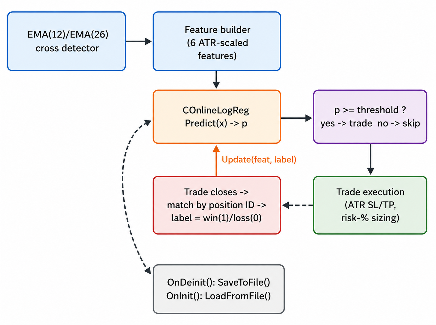
Fig. 1. Data flow through the EA: signal detection, feature construction, the online model, the threshold gate, trade execution, and the closed-trade label written back into the model.

The base signal is deliberately plain, an EMA(12)/EMA(26) cross checked once per new bar; anything you already trade with a binary "would I have entered here" moment fits the same slot:

int CheckCrossSignal()
  {
   double ema_f[2], ema_s[2];
   CopyBuffer(h_ema_fast, 0, 1, 2, ema_f);
   CopyBuffer(h_ema_slow, 0, 1, 2, ema_s);

   bool cross_up   = (ema_f[0] <= ema_s[0]) && (ema_f[1] > ema_s[1]);
   bool cross_down = (ema_f[0] >= ema_s[0]) && (ema_f[1] < ema_s[1]);

   if(cross_up)    return(1);
   if(cross_down) return(-1);
   return(0);
  }

Six features are built from the just-closed bar, each scaled explicitly rather than left implicit:

x0 = RSI(14) / 100    x1 = (close - EMAslow) / ATRfast    x2 = ATRfast / ATRslow
x3 = (close - open) / (high - low)    x4 = (MACDmain - MACDsignal) / ATRfast    x5 = volume / SMA(volume, 20)

Every one of these exists to put six otherwise incomparable quantities onto a common footing before a gradient update; skip the scaling and the largest-magnitude feature dominates regardless of how informative it actually is. The construction itself:

bool BuildFeatures(double &feat[])
  {
   double ema_f[1], ema_s[1], rsi_v[1], atr_f[1], atr_s[1],
         macd_main[1], macd_sig[1], vol_sma[1];

   if(CopyBuffer(h_ema_fast, 0, 1, 1, ema_f) <= 0) return(false);
   if(CopyBuffer(h_ema_slow, 0, 1, 1, ema_s) <= 0) return(false);
   if(CopyBuffer(h_rsi,      0, 1, 1, rsi_v) <= 0) return(false);
   if(CopyBuffer(h_atr_fast, 0, 1, 1, atr_f) <= 0) return(false);
   if(CopyBuffer(h_atr_slow, 0, 1, 1, atr_s) <= 0) return(false);
   if(CopyBuffer(h_macd, 0, 1, 1, macd_main) <= 0) return(false);
   if(CopyBuffer(h_macd, 1, 1, 1, macd_sig)  <= 0) return(false);
   if(CopyBuffer(h_vol_sma,  0, 1, 1, vol_sma) <= 0) return(false);

   double close1 = iClose(_Symbol, PERIOD_CURRENT, 1);
   double open1  = iOpen(_Symbol, PERIOD_CURRENT, 1);
   double high1  = iHigh(_Symbol, PERIOD_CURRENT, 1);
   double low1   = iLow(_Symbol, PERIOD_CURRENT, 1);
   long   vol1   = iVolume(_Symbol, PERIOD_CURRENT, 1);
   if(atr_f[0] <= 0.0 || atr_s[0] <= 0.0) return(false);

   ArrayResize(feat, N_FEATURES);
   feat[0] = rsi_v[0] / 100.0;
   feat[1] = (close1 - ema_s[0]) / atr_f[0];
   feat[2] = atr_f[0] / atr_s[0];
   double range = high1 - low1;
   feat[3] = (range > 0.0) ? (close1 - open1) / range : 0.0;
   feat[4] = (macd_main[0] - macd_sig[0]) / atr_f[0];
   feat[5] = (vol_sma[0] > 0.0) ? (double)vol1 / vol_sma[0] : 1.0;
   return(true);
  }

Every buffer read and the ATR values are checked before use, and the function simply skips the signal on a bad read rather than training the model on a division-by-zero artifact.

This is a deliberately minimal feature set, a reasonable starter pack rather than a systematically engineered one. It has no interaction terms, no explicit long/short asymmetry, and no contextual variables like session or spread regime. Extending it is straightforward given the scaling discipline above, but the choice here optimizes for auditability over completeness. The same reasoning shapes the choice of model: logistic regression is linear, cheap, and trivially online-updatable, not the strongest classifier available. We are choosing the minimally sufficient, controllable adaptive classifier for this job, not "the best ML."

The filter's entire job is one comparison:

double prob = model.Predict(feat);
if(prob < InpProbThreshold)
   return; // the filter vetoes this base signal

Closing the loop after the trade is placed is the part a static ML article never has to deal with. The EA keeps a small pending-samples array, keyed by DEAL_POSITION_ID rather than a deal ticket so partial closes and netting/hedging modifications don't break the mapping. It's filled the moment a trade is sent:

PendingPush(pos_id, feat);

Every tick, ProcessClosedTrades() finds any closed position not yet labeled, computes profit including swap and commission, a trade green on price but net negative after cost should train as a loss, and updates the model:

double profit = HistoryDealGetDouble(deal_ticket, DEAL_PROFIT)
               + HistoryDealGetDouble(deal_ticket, DEAL_SWAP)
               + HistoryDealGetDouble(deal_ticket, DEAL_COMMISSION);
int label = (profit > 0.0) ? 1 : 0;
model.Update(feat, label);

Position sizing is fixed-fractional off the ATR-based stop distance, rounded to the broker's lot step and clamped to min/max volume:

lots = R / ( (D / tick_size) · tick_value ),   R = balance · (risk_percent / 100)

Stop and take-profit are ATR multiples, 1.5 and 2.5 by default, rather than fixed pips, so the same EA behaves sensibly across symbols with very different pip values instead of quietly assuming one.

Seeing it learn: the probability indicator

OnlineML_ProbabilityView.mq5 is a read-only window onto the same weights the EA is training: it loads the EA's saved CSV, reconstructs a COnlineLogReg instance, and plots Predict() for each historical bar's feature vector in a sub-window. It never calls Update() and never trades.

One interpretation caveat matters specifically here. Because the indicator reconstructs weights that were learned later and applies them back across history, what it plots is a retrospective probability, not the live forward probability the EA actually acted on at that bar in real time. A bar in the middle of the chart can show a confident line even though the model, at that point historically, hadn't learned enough yet to justify it. Don't read the indicator's historical shape as "what the model thought back then." Section 15 covers the related cold-start caution in more detail.

The evidence: does it actually separate winners from losers

A claim that "the model learns" needs a number attached to it. A controlled setting gives a cleaner one than a live chart ever could, since we never know the true relationship between a real market's features and its outcomes. OnlineML_SyntheticEvidence.mq5 generates six-feature vectors from a known, deliberately noisy linear relationship and feeds them one at a time into a fresh COnlineLogReg. Each sample is scored in a rolling 100-trade window before that trade's own label updates the model, an honest out-of-sample check:

double p_before = model.Predict(f); // scored before this trade's label is known
// ... record (p_before, y) into the rolling window ...
model.Update(f, y);

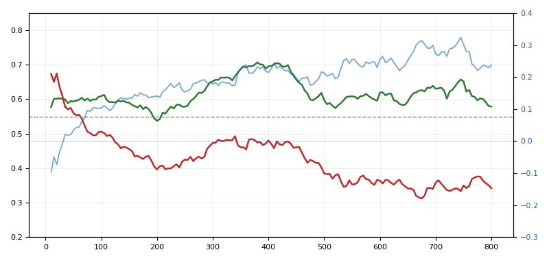
Fig. 2. Model probability on winners (green) vs. losers (red) over 800 trades, separation on the right axis, dashed line at the 0.55 threshold.

Table 1 is one run at η=0.05:

Trades	avg P | win	avg P | loss	separation	precision @ 0.55
10	0.578	0.674	-0.096	0.833
25	0.603	0.636	-0.033	0.700
50	0.594	0.560	+0.034	0.719
100	0.609	0.506	+0.104	0.754
200	0.538	0.397	+0.141	0.600
400	0.696	0.480	+0.215	0.734
800	0.579	0.342	+0.237	0.730

Table 1. Synthetic separation sweep, 6-feature noisy linear generator, 100-trade rolling window, η=0.05.

Precision@0.55 reads 0.833 at trade 10, high, right where separation is most negative, but that's from only six trades in the window, not a sign the filter already works; from the 100-trade checkpoint on it settles into the 0.70-0.75 range Table 1's trend actually supports.

Separation starts negative (-0.096 at trade 10), crosses positive between trades 25-50, and climbs to +0.237 by trade 800, not perfectly monotonic, but the trend across checkpoints is the evidence. In short: unreliable for roughly the first 25-50 trades, increasingly useful after.

Table 1 is one seed, and one seed is an anecdote, not evidence, so OnlineML_SyntheticEvidence.mq5 now also runs the same 800-trade experiment across 200 independent seeds and reports the spread, not just a single number:

Metric	Value
Mean separation @ trade 800	+0.233
Standard deviation	0.051
95% interval (2.5–97.5 percentile)	[+0.141, +0.334]
Seeds with positive separation	200 / 200 (100%)

Table 1b. Separation at trade 800 across 200 independent seeds, same generator and hyperparameters as Table 1.

Table 1 wasn't a lucky draw: the single-seed +0.237 sits almost exactly on the 200-seed mean of +0.233, and the interval never crosses zero, all 200 runs ended positive.

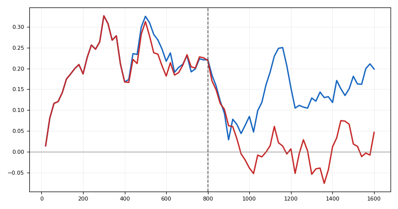
Fig. 3. All six learned weights over the same 800-trade run, against their true generative values.

Figure 3 shows the same run's six weights against their true generative values: four settle into a reasonably stable band, two overshoot and keep drifting, and one, the ATR-ratio feature, is still moving at trade 800 rather than converged. This is single-sample SGD's variance on a noisy problem, not a batch method's clean convergence to one fixed answer, and it is the gap Section 10's learning-rate decay is meant to narrow.

Feature ablation: why these six

Section 4 listed six features without saying which carry the signal. OnlineML_SyntheticEvidence.mq5 now re-runs the 800-trade experiment with each feature zeroed out, 50 seeds per configuration:

Configuration	Mean sep. @ 800	Δ vs. all six
All six features	+0.222	—
Drop EMA-dist/ATR (x1)	+0.074	-0.148
Drop MACD hist/ATR (x4)	+0.153	-0.069
Drop any of the other four	+0.212 to +0.222	< 0.01
Trend-only (x1, x3, x4)	+0.221	-0.001
Volatility/context-only (x0, x2, x5)	-0.004	-0.226

Table 2. Feature ablation, 50 seeds per configuration, 800-trade synthetic generator.

Two features, x1 and x4, carry almost all the signal in this synthetic generator; dropping any of the other four costs less than 0.01, noise-level at this seed count. This tracks the generator's own design: x1 and x4 carry the largest true weights, so the ablation recovers the ranking built into the data. That's the honest limit of it, too: this validates the test harness on a problem with a known answer. It is not feature importance on EURUSD or any real symbol, and needs re-running against real trade outcomes once Section 13's validation loop has produced them.

Calibration: is this a meaningful probability?

Calling this a "probability filter" is a stronger claim than "a score good enough to threshold": that 0.70 really means close to 7 wins in 10. Checked directly, using out-of-sample p_before from Table 1's run, trade 200 onward:

Metric	Value	Reading
ROC-AUC	0.771	Well above 0.5; the model ranks winners above losers most of the time.
Brier score	0.194	Below the 0.25 a coin-flip-at-the-base-rate model would score.
Log-loss	0.570	Reasonable for a base rate near 0.48; not directly comparable across problems.

Table 3. Calibration metrics, single run, trades 200-800, n≈12,000 pooled across 20 seeds.

None of those three numbers alone proves calibration; a reliability table does, by checking whether trades the model scored around 0.70 actually won about 70% of the time:

Predicted bin	n	Actual win rate	Avg. predicted
[0.30, 0.40)	1,579	0.355	0.351
[0.40, 0.45)	760	0.434	0.425
[0.45, 0.50)	778	0.479	0.475
[0.50, 0.55)	723	0.510	0.525
[0.55, 0.60)	775	0.560	0.576
[0.60, 0.65)	735	0.626	0.625
[0.65, 0.70)	696	0.682	0.675
[0.70, 0.80)	1,214	0.739	0.749

Table 4. Reliability table: predicted-probability bin vs. actual win rate in that bin.

Every bin's actual win rate sits within about a point of its average predicted probability, monotonic across all eight bins, "0.75" really does mean close to 75% here. This is a different question from separation: a model can rank winners above losers perfectly while still being miscalibrated (e.g. always predicting 0.9/0.6 when true rates are 0.6/0.3). Table 4 rules that out on the generator; it does not rule it out on a real instrument, where this same table needs rebuilding from real trade history before any threshold can be trusted as a real probability. One caveat worth stating plainly: the generator itself is logistic in form, linear in the features plus noise, which is a favorable setting for a logistic-regression model almost by construction. This section verifies the implementation behaves correctly, not that real-market calibration is achievable; a real instrument gives no such guarantee.

Static vs. online under a regime shift, with two more baselines

Section 2 told this as an argument; this section runs it as an experiment, with four models now, not two. The extremes: an online model calling Update() every trade, and a frozen baseline, trained for 400 trades then never again. Between them: a periodic model, batch-retrained on all history every 200 trades, and a rolling model, batch-retrained on the trailing 400 trades every 50. Periodic and rolling never call the online update, both represent "retrain occasionally," at different scopes, the middle ground a two-model comparison alone would leave untested.

All four see the same relationship for the first 800 trades; at trade 800 the generator switches to a second relationship where two feature weights flip sign and the bias shifts:

// regime A (trades 1..800), matches the base evidence test
double regimeA_w[6] = {0.9, 1.3, -0.4, 0.6, 1.1, 0.3};
double regimeA_b = -0.6;

// regime B (trades 801..1600): x1 and x3 flip sign, the bias moves
double regimeB_w[6] = {0.9, -1.1, -0.4, -0.7, 1.1, 0.3};
double regimeB_b = 0.1;

Freezing is one line, not calling a function again; periodic and rolling batch-train a fresh model over several epochs on a window of history, each on its own cadence.

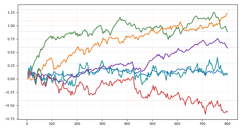
Fig. 4. Horizontal axis: labeled trades seen, 0 to 1600. Vertical axis: rolling 100-trade win/loss probability separation, for online (blue), frozen at trade 400 (red), periodic retrain every 200 trades (orange), and rolling 400-trade retrain (green). Dashed vertical line marks the regime shift at trade 800.

Trade	online	frozen	periodic (200)	rolling (400)
600	+0.224	+0.220	+0.242	+0.242
800	+0.224	+0.218	+0.242	+0.238
-- regime shift --
900	+0.025	-0.074	-0.063	-0.011
1000	+0.134	-0.072	-0.062	+0.127
1200	+0.184	-0.068	+0.162	+0.196
1600	+0.206	-0.067	+0.210	+0.217

Table 5. Mean win/loss probability separation across 30 seeds, before and after the regime shift at trade 800, for all four policies.

All four are close pre-shift (periodic and rolling land slightly ahead from multiple epochs over their window). Separation collapses for all four by trade 900, then splits: frozen never recovers, still -0.067 at trade 1600. Periodic recovers slowly, at trade 1000 it's still negative, since a retrain on all 1,000 trades is diluted by 800 stale regime-A examples against 200 fresh ones, and only turns positive once regime-B accumulates enough weight. Online and rolling recover fastest, online because every trade nudges it, rolling because its 400-trade window fully flips to regime-B well before trade 1600.

Online SGD isn't the only way to survive a regime shift, rolling gets there about as fast here, periodic gets there eventually but slower, dragged down by a growing pile of outdated examples. What every non-frozen policy shares is a mechanism for old-regime evidence to stop dominating; the frozen baseline permanently lacks exactly that.

Extending the model: a decaying learning rate

Figure 3 showed weights that never quite settle, a direct consequence of a fixed η treating trade 1 and trade 800 identically. SetLearningRateDecay(decay, floor) shrinks η a little after every update down to a floor that keeps it from ever fully freezing, which would just reproduce the baseline's failure mode above. Wiring it in is one call after Init():

model.Init(N_FEATURES, InpLearningRate, InpL2Lambda);
model.SetLearningRateDecay(0.001, 0.01); // 0.1% shrink per update, floor at 0.01

A decay of 0.001 with a floor of 0.01 takes η from 0.05 down to roughly 0.018 by trade 1000, a gentle taper rather than a cliff; the floor matters because decaying all the way toward zero would eventually reproduce the frozen baseline's problem, just more slowly.

This is off by default in the EA, purely so the numbers in Sections 7 and 10 stay unambiguous. Turning it on shifts every one of those numbers. The cold-start length, the regime-shift recovery time, and the weight-trajectory noise band all move together, so re-run the relevant script with decay enabled before trusting a decayed configuration, rather than assuming the undecayed figures still apply.

Hyperparameter sensitivity

Does the result need η=0.05 exactly, or hold across a range? 20 seeds per point:

η (L2=0.0005)	Sep@800	λ (η=0.05)	Sep@800
0.01	+0.170	0.0000	+0.237
0.05 (default)	+0.237	0.0005 (default)	+0.237
0.10	+0.243	0.0100	+0.223
0.30	+0.242	0.0500	+0.183

Table 6. Learning-rate and L2 sweeps, 20 seeds/point, full range in the script.

Separation is flat from η=0.05 to 0.30, softening only below 0.02; L2 barely matters below 10× the default. Both defaults sit in a flat, safe region. The threshold is a trading decision, not a training one, with a real, monotonic trade-off (pooled sample from Section 8):

Threshold	Trade rate	Precision
0.50	46.1%	0.690
0.55 (default)	40.1%	0.718
0.60	33.6%	0.748
0.65	27.5%	0.775

Table 7. Threshold sweep, pooled sample (n=12,020).

Precision rises and trade count falls monotonically with threshold, as a calibrated model should. 0.55 is a reasonable middle point, not a discovered optimum; the right value depends on real cost, which only Section 13's real test can reveal.

Label design and alternatives

Every result here trains on label = (profit > 0.0) ? 1 : 0, the simplest label that works. It throws away magnitude: 0.01R and 3R both get label=1, -0.05R and -3R both get label=0. Three alternatives exist, none implemented in the attached code. R-multiple: a continuous label, profit/risk, with a regression loss, answers "how good relative to risk." Cost-adjusted threshold: move the cutoff from profit>0 to profit>expected_cost, a one-line change. Triple-barrier: label by whichever of a fixed TP, fixed stop, or max hold time hits first, independent of the EA's own exit logic. R-multiple suits ranking signal quality, cost-adjusted suits avoiding clearly unprofitable trades, triple-barrier suits comparing against a different exit scheme. Whichever is chosen, re-run Section 7's ablation and Section 8's calibration against the new label; both were validated only against the crude binary label used here.

Validating this on your own instrument

Table 1 establishes the algorithmic claim; it says nothing about whether an EMA cross has any exploitable relationship to these six features on a real symbol. One backtest doesn't answer that either, one run on one period is the anecdote Section 6's multi-seed table exists to avoid, so this is a walk-forward protocol, not a single Tester click. Split history into chronological train (weights warm up, saved), validation (pick the threshold), and forward (touched exactly once, never re-tuned) blocks, then roll all three ahead and repeat: train on months 1-6, validate on 7, forward-test on 8; then 2-7 / 8 / 9; and so on. A filter that clears its bar on one slice and fails on others is overfit to that slice, not to the market.

Inside each fold:

• Run OnlineML_SignalFilter_EA at InpProbThreshold = 0.0 (unfiltered) and again at 0.55 (filtered), everything else identical.
• Compare total trades, win rate, profit factor, and max drawdown.
• Use real-tick mode, not default OHLC simulation; test more than one symbol; run long enough to clear cold start.

Before trusting the filtered version, check, in every fold: trade count didn't collapse past usefulness (60-80% reduction is reasonable, 98% is a broken threshold); win rate improved after real costs, not just raw P/L; profit factor didn't worsen; drawdown isn't materially worse. The improvement should also hold across at least two adjacent periods, not just one. Report the spread across folds, not just the average, a profit factor of 1.4 that ranges 1.1-1.7 across folds is a weaker claim than 1.4 in every fold.

A filter that fails any of these checks, in any fold, isn't automatically worthless. It just isn't ready to trust yet. Section 15's pitfalls are usually more productive to revisit than adjusting the threshold by feel. I haven't published this comparison myself yet, see the introduction's scope note.

Operational notes: running this live

Three things beyond the mechanism itself matter once this runs unattended: keeping the weights file honest, avoiding leakage, and knowing where to start.

Weights file hygiene. OnDeinit() saves on normal shutdown only, not a crash; add a periodic save (every N trades or on a timer) for anything beyond a demo test. After LoadFromFile(), sanity-check the loaded weights (reject NaN, infinite, or wildly out-of-range values and cold-start instead of trading on a corrupted vector). Encode symbol and timeframe into the filename, e.g. OnlineML_weights_EURUSD_H1.csv, since nothing else stops you loading the wrong instrument's weights. Bump a version number whenever BuildFeatures()'s feature set changes shape or order, and treat any change to trade-management logic, not just features, as a reason to cold-start.

Leakage and tester-mode checks. BuildFeatures() always reads shift 1 (the last closed bar), never shift 0, so feature and entry timing stay synchronized. The label is only known once a trade closes, so the most recent few trades are always unlabeled, correct behavior, not a bug. Use "every tick based on real ticks" tester mode, not default OHLC simulation. ProcessClosedTrades() trains directly on whatever profit the Tester reports, so an optimistic fill model inflates the labels, not just the P/L; slippage and partial fills bias which signals get labeled as wins through that same channel.

Where to start. Leave η=0.05 and L2=0.0005 alone (Section 11's sweep), start the threshold at 0.55 and move it only after a walk-forward comparison at the candidate value. Treat fewer than 100 labeled trades as still cold-start regardless of how it looks. Reset the model after any logic change, after a sustained negative rolling-separation stretch, or after a weights-version mismatch. Pre-training in the Tester is fine; validating on the same window you pre-trained on is not, always walk-forward to a later window. Log per trade, at minimum: timestamp, symbol, timeframe, the six features, predicted probability, whether taken, eventual label, realized profit including costs, and current learning rate. This feeds drift diagnosis, and lets Section 7's ablation and Section 8's calibration checks be re-run against real trades later.

Edge cases and pitfalls

Online ≠ profitable. Table 1 shows the update rule can separate a controlled, known relationship from noise. It says nothing about whether your instrument's crossover has any real relationship to these six features; if it doesn't, no amount of online adaptation fixes a feature set with no signal in it.

Cold start costs real trades. At all-zero weights the model outputs a flat 0.5 for every signal, so the first stretch of trades above threshold is close to unfiltered. Pre-train in the Strategy Tester and load the resulting weights file if you want to avoid paying this cost in real money on a live account; Section 14 has the pre-training-without-fooling-yourself caveat.

A fixed learning rate for the whole lifetime is a simplification. Section 10's optional decay addresses this; it is off by default to keep the article's core numbers unambiguous.

Feature scaling is manual.COnlineLogReg does no normalization itself; keep any feature you add on a comparable scale, or SGD will let the largest-magnitude feature dominate the gradient regardless of how informative it actually is.

Match by position ID, not order ticket. DEAL_POSITION_ID survives partial closes and netting/hedging modifications; a deal ticket doesn't. Keep matching on it if you extend the EA to scale in or out of a position.

The synthetic scripts use their own RNG, not MathRand(). Both evidence scripts implement a small linear congruential generator so a given seed reproduces the same sequence across terminal builds; this only matters for reproducibility of the test, not the live EA.

Periodic and rolling retraining are batch stand-ins, not deployable pipelines. Section 9's baselines are batch passes inside a script, not an automated offline-retrain-and-redeploy workflow; building that is separate engineering work.

A decayed learning rate invalidates the undecayed numbers. Every figure in Sections 7, 9, and 10 was produced without decay; re-run the relevant script before trusting a decayed configuration.

The label, profit > 0, is crude, and it isn't just noted here anymore. Section 12 covers what it throws away and three concrete alternatives (R-multiple, cost-adjusted threshold, triple-barrier), none implemented in the attached code.

No class-imbalance handling. If wins and losses aren't roughly balanced in your history, a flat 0.55 threshold may be naive; check the base rate on your instrument before trusting it as-is.

Calibration is checked on synthetic data only. Section 8's ROC-AUC, Brier score, and reliability table establish that the model's outputs are a meaningful probability on the generator. They say nothing yet about calibration on real trade history, which needs its own reliability table built from Section 14's logged predictions.

The model is linear in the features. It cannot capture interactions or nonlinearities without you engineering them in explicitly. That is a deliberate trade for simplicity and online-updatability, not a claim that logistic regression is the strongest classifier available for this job. Section 7's ablation is the closest this article comes to testing whether that trade costs anything on this particular problem.

Batch retraining has a real cost at high frequency. Periodic/rolling retrain is O(epochs × window size) per retrain; seconds in a script, worth profiling before deploying on a live EA at high retrain frequency.

Conclusion

This article built an online logistic regression filter for MQL5: a shared class (OnlineLogReg.mqh, now with optional decay), an EA that trades EMA-cross signals against it and feeds outcomes back in, and a read-only visualization. Two synthetic test scripts back it up, now covering multi-seed statistics, feature ablation, calibration, hyperparameter sweeps, and four regime-shift baselines instead of one comparison.

What's proven, with error bars instead of anecdotes: separation of +0.233 mean at trade 800 across 200 seeds, 95% CI [+0.141, +0.334], never crossing zero. Two of six features (EMA-dist/ATR, MACD-hist/ATR) carry essentially all the signal. Outputs are calibrated (ROC-AUC 0.771, reliability agreeing within ~1pt across bins), not just separated. Online recovers from a regime shift that leaves frozen stuck negative; periodic and rolling retraining also recover, just slower. All of it holds across a wide learning-rate and L2 range. These are algorithmic and architectural claims, each backed by a re-runnable script.

What isn't proven: that these features or this label carry a real, cost-resistant edge on any instrument. That's a trading claim, open until Section 13's walk-forward runs on real tick data.

A concrete Part 2: everything here is synthetic; the real-market counterpart, not a new mechanism, would be EURUSD H1, five years of real tick data, walk-forward folds per Section 13; filtered vs. unfiltered on that same protocol; the Section 11 threshold sweep against real precision and cost; a slippage/cost stress test; multi-symbol robustness (GBPUSD, XAUUSD, an index); and the Section 7 ablation and Section 8 calibration re-run against real labeled trades. The file table below has everything needed to build, test, and extend it.

File	Type	Description
OnlineLogReg.mqh	Library	The COnlineLogReg class: sigmoid forward pass, per-sample SGD update with L2 regularization, optional learning-rate decay, and CSV save/load persistence.
OnlineML_SignalFilter_EA.mq5	Expert Advisor	EMA crossover signal, six-feature construction, probability-threshold filtering, ATR-based trade management, and the closed-trade feedback loop that labels and updates the model.
OnlineML_ProbabilityView.mq5	Indicator	Read-only sub-window plot of the model's win-probability estimate, loaded from the EA's saved weights file.
OnlineML_SyntheticEvidence.mq5	Script	v2.00: single-seed checkpoint table, plus a 200-seed statistical summary, six-way feature ablation (50 seeds each), and calibration diagnostics (ROC-AUC, Brier, log-loss, reliability table).
OnlineML_RegimeShift_Evidence.mq5	Script	v2.00: compares four policies across a regime shift, online, frozen, periodic (all-history batch retrain), and rolling (400-trade window retrain), with a single-seed printout and a 30-seed summary table.
MQL5.zip	Archive	Archive with all five source files above plus the figure images. Unpack it into the terminal installation directory and every file is placed in its required location.