Market Microstructure in MQL5 (Part 6): Order Flow

MetaTrader 5 — Indicators | 23 June 2026, 08:45

257

Max Brown

Introduction

Part 1 built the defensive foundation. Part 2 and Part 3 measured whether price has memory. Part 4 measured what volatility is doing and whether it persists. Part 5 decomposed price variation into noise and signal. Part 6 asks the final measurement question: which direction is the informed flow moving?

Order flow is the proximate cause of price changes. Every price movement results from one side of the market being more aggressive than the other — buyers lifting offers or sellers hitting bids. The challenge at one-minute resolution is that the aggressor side is not directly observable from OHLCV data. The functions in this article construct bar-level approximations of order flow. They are conditioned on the noise and volatility measures from Parts 4 and 5. The output is connected to the OrderFlowSignal struct reserved in Part 1.

Before the implementation sections, two points require explicit framing — both involve the same M1 aggregation problem documented in Part 5.

VPIN_OHLC() approximates the volume-imbalance component of the Easley, López de Prado and O'Hara (2012) VPIN measure using bar-level data. The canonical VPIN requires fixed-volume buckets where every trade contributes to the imbalance estimate. On one-minute NQ futures bars, each bar contains hundreds of executions. For the same reason as the Roll spread in Part 5, intrabar aggregation absorbs the microstructure signal, so the imbalance collapses toward 0.5. The empirical study shows a total VPIN range of 0.45 to 0.62 across 602 sessions, with regime elevations of 6% during stress. This is a weak but directionally correct signal. It is retained as the OHLCV-best-available approximation and must not be interpreted as a statistically calibrated probability of informed trading.

TradeIntensity() compares current session volume to a 20-session rolling baseline. The first 20 sessions of the dataset produce inflated ratios because the baseline is still warming up. In the empirical study, this produces a single extreme outlier (1,250×) on the first session. The reported statistics use values winsorized at the 99th percentile (1.63×); this is documented in the empirical section.

Deliverable: six functions added to MicroStructure_Foundation.mqh, a new OrderFlowAnalysis struct, and the flow signal connected to the noise and volatility outputs from Parts 4 and 5. No new include file is created. The companion SSRN paper is available at SSRN 6847024.

The Theory of Order Flow

Order flow and price impact

Kyle (1985) showed that informed traders camouflage their orders within the noise flow, and that prices adjust as market makers infer the information content of the order stream. The key insight is that the direction and magnitude of volume imbalance — the excess of buy volume over sell volume — is the observable footprint of informed activity. When buyers are more aggressive than sellers, prices rise. When sellers dominate, prices fall. The rate of price change per unit of signed order flow is the Kyle lambda — the price impact coefficient.

At tick level, the aggressor side of each trade is directly observable: a buy is a trade executed at the ask, a sell is a trade executed at the bid. At bar level, it must be inferred. The standard inference rule — used by VPIN, by the Lee-Ready (1991) algorithm, and by the OHLCV proxy here — is that bars closing near their high are buyer-dominated and bars closing near their low are seller-dominated. This inference is correct in expectation but noisy in individual bars, which is why bar-level order flow measures carry wider confidence intervals than tick-level equivalents.

VPIN — Volume-Synchronized Probability of Informed Trading

Easley, López de Prado and O'Hara (2012) proposed VPIN as a real-time measure of order flow toxicity. The canonical definition uses fixed-volume buckets: each bucket represents a fixed quantity of market activity, and the imbalance between buy and sell volume within each bucket measures the probability that at least one counterparty in that bucket was informed. The key property is that VPIN is stationary in activity rather than in clock time — a bucket represents the same amount of market participation regardless of whether it takes 10 seconds or 10 minutes to fill.

The OHLCV approximation implemented here — VPIN_OHLC() — replaces volume buckets with fixed time bars. This approximation loses the stationarity property but preserves the directional signal. The function is an honest first-order estimate of the imbalance fraction, with the limitation stated prominently in the function header and the empirical section.

Smart money index

The Smart Money Index identifies the intraday pattern where large informed participants tend to act in the final portion of the session, after the noise-driven opening volatility has dissipated. Early-session price moves are dominated by retail flow, news reactions, and stop-running activity. Late-session moves are more likely to reflect institutional positioning. A session where price falls early and then recovers late — positive SMI — suggests informed accumulation. A session where price rises early and then weakens late — negative SMI — suggests institutional distribution.

Trade intensity

Trade intensity measures whether the current session's volume is elevated relative to the recent baseline. High relative volume indicates that more participants are active — consistent with informed flow, news events, or both. Low relative volume indicates a quiet session where the OHLCV flow proxies are less reliable because there are fewer trades to aggregate.

Connection to Parts 4 and 5

The connection between Part 6 and the earlier articles is explicit and bidirectional. The noise ratio from Part 5 gates the flow_confidence weight: when noise is elevated above the 75th percentile (0.632), the VPIN and imbalance estimates are less reliable because the volume proxy for aggressor side is contaminated by the same transient friction that distorts the price. The jump intensity from Part 4 sets flow_confidence to zero when it exceeds the 90th percentile (2.1%) — jump-contaminated sessions should not be traded on flow signals. The clustering index from Part 4 is the recommended conditioning variable for flow momentum: order flow momentum is more persistent when volatility is clustered.

Implementation

New struct: OrderFlowAnalysis

//+------------------------------------------------------------------+
//| OrderFlowAnalysis: order flow measurement results.               |
//| Populated by PopulateOrderFlowAnalysis().                        |
//| flow_confidence is gated on noise (Part 5) and jump intensity    |
//| (Part 4). It is zero when the session is jump-contaminated.      |
//+------------------------------------------------------------------+
struct OrderFlowAnalysis
  {
   double vpin;               // VPIN_OHLC: volume imbalance proxy [0,1]
   double flow_imbalance;     // Signed volume-weighted directional flow [-1,+1]
   double trade_intensity;    // Session vol relative to 20-session baseline
   double smart_money;        // Late-session minus early-session return differential
   double flow_momentum;      // Short-window minus long-window flow differential
   double flow_confidence;    // Reliability weight [0,1]; 0 = jump-contaminated
  };

VPIN_OHLC()

For each bar, the buy volume proxy is (Close − Low)/(High − Low) × Volume and the sell volume proxy is the complement. VPIN is the mean absolute imbalance fraction normalized by total volume over the window. Returns a value in [0, 1]. Values above the 75th percentile (0.539) indicate elevated directional imbalance; values above the 90th percentile (0.559) indicate strong imbalance. The function header explicitly states this is an OHLCV approximation and should not be interpreted as the calibrated VPIN probability of Easley et al. (2012).

//+------------------------------------------------------------------+
//| VPIN_OHLC: volume imbalance proxy over a rolling window.         |
//| buy_vol  = (Close-Low)/(High-Low) * Volume                       |
//| sell_vol = (1-(Close-Low)/(High-Low)) * Volume                   |
//| VPIN = mean(|buy-sell|) / mean(total vol) across the window.     |
//|                                                                  |
//| THIS IS NOT THE EASLEY-LOPEZ DE PRADO-O'HARA VPIN.               |
//| The canonical VPIN uses fixed-volume buckets, not fixed time     |
//| bars. On NQ M1, intrabar aggregation compresses the imbalance    |
//| signal toward 0.5. Treat as a directional indicator only.        |
//+------------------------------------------------------------------+
double VPIN_OHLC(const string symbol, const int tf,
                  const int window)
  {
   if(!ValidateSymbolV2(symbol) || window < 5) return 0.5;
   double high[], low[], close[];
   long   vol[];
   ArraySetAsSeries(high,true); ArraySetAsSeries(low,true);
   ArraySetAsSeries(close,true); ArraySetAsSeries(vol,true);
   if(CopyHigh     (symbol,(ENUM_TIMEFRAMES)tf,0,window,high)  < window) return 0.5;
   if(CopyLow      (symbol,(ENUM_TIMEFRAMES)tf,0,window,low)   < window) return 0.5;
   if(SafeCopyClose(symbol,tf,0,window,close)                  < window) return 0.5;
   if(CopyTickVolume(symbol,(ENUM_TIMEFRAMES)tf,0,window,vol)  < window) return 0.5;
   double sum_imb = 0.0, sum_vol = 0.0;
   for(int i = 0; i < window; i++)
     {
      double br = high[i] - low[i];
      if(br <= DBL_MIN_POSITIVE) continue;
      double v    = (vol[i] > 0) ? (double)vol[i] : 1.0;
      double frac = MathMax(0.0, MathMin(1.0,
                             (close[i] - low[i]) / br));
      double buy_v  = frac * v;
      double sell_v = (1.0 - frac) * v;
      sum_imb += MathAbs(buy_v - sell_v);
      sum_vol += v;
     }
   if(sum_vol <= DBL_MIN_POSITIVE) return 0.5;
   return MathMax(0.0, MathMin(1.0, sum_imb / sum_vol));
  }

OrderFlowImbalance()

Signed volume-weighted directional flow. Extends Part 5's OrderImbalance() by preserving the magnitude of the deviation from 0.5, which makes the signed result more sensitive to strong directional bars. Returns values in [−1, +1].

//+------------------------------------------------------------------+
//| OrderFlowImbalance: signed volume-weighted directional flow.     |
//| Each bar: signed_imb = ((Close-Low)/(High-Low) - 0.5) * 2 * vol  |
//| Returns sum(signed_imb) / sum(vol) in [-1,+1].                   |
//| +1 = all closes at high (buyer dominated).                       |
//| -1 = all closes at low (seller dominated).                       |
//+------------------------------------------------------------------+
double OrderFlowImbalance(const string symbol, const int tf,
                           const int window)
  {
   if(!ValidateSymbolV2(symbol) || window < 3) return 0.0;
   double high[], low[], close[];
   long   vol[];
   ArraySetAsSeries(high,true); ArraySetAsSeries(low,true);
   ArraySetAsSeries(close,true); ArraySetAsSeries(vol,true);
   if(CopyHigh     (symbol,(ENUM_TIMEFRAMES)tf,0,window,high)  < window) return 0.0;
   if(CopyLow      (symbol,(ENUM_TIMEFRAMES)tf,0,window,low)   < window) return 0.0;
   if(SafeCopyClose(symbol,tf,0,window,close)                  < window) return 0.0;
   if(CopyTickVolume(symbol,(ENUM_TIMEFRAMES)tf,0,window,vol)  < window) return 0.0;
   double weighted_sum = 0.0, total_vol = 0.0;
   for(int i = 0; i < window; i++)
     {
      double br = high[i] - low[i];
      if(br <= DBL_MIN_POSITIVE) continue;
      double frac = MathMax(0.0, MathMin(1.0,
                             (close[i] - low[i]) / br));
      double v   = (vol[i] > 0) ? (double)vol[i] : 1.0;
      weighted_sum += (frac - 0.5) * 2.0 * v;
      total_vol    += v;
     }
   if(total_vol <= DBL_MIN_POSITIVE) return 0.0;
   return MathMax(-1.0, MathMin(1.0, weighted_sum / total_vol));
  }

TradeIntensity()

Computes mean bar volume for the current window and divides by the cached baseline. The baseline must be supplied by the caller from a longer historical window — typically 20 sessions of mean bar volume. This design keeps the function stateless and testable. Values above 1.0 indicate above-average activity; the 75th percentile (1.13×) is the recommended threshold for elevated activity on NQ M1.

//+------------------------------------------------------------------+
//| TradeIntensity: current vol relative to historical baseline.     |
//| Returns mean_volume(window) / baseline.                          |
//| baseline must be pre-computed from a longer lookback (caller).   |
//| Values above 1.0 = above-average activity.                       |
//| NOTE: baseline requires at least 20 sessions to be meaningful.   |
//| The first 20 sessions after data start will produce inflated     |
//| values as the baseline warms up. Check baseline > 1 before use.  |
//+------------------------------------------------------------------+
double TradeIntensity(const string symbol, const int tf,
                       const int window, double baseline)
  {
   if(!ValidateSymbolV2(symbol) || window < 2
      || baseline <= DBL_MIN_POSITIVE) return 1.0;
   long vol[];
   ArraySetAsSeries(vol, true);
   if(CopyTickVolume(symbol,(ENUM_TIMEFRAMES)tf,0,window,vol) < window)
      return 1.0;
   double sum_v = 0.0;
   int    valid = 0;
   for(int i = 0; i < window; i++)
      if(vol[i] > 0) { sum_v += (double)vol[i]; valid++; }
   if(valid == 0) return 1.0;
   return MathMax(0.0, (sum_v / valid) / baseline);
  }

SmartMoneyIndex()

Computes the log-return in the first N bars of the available window (early, noise-dominated) and the log-return in the final N bars (late, informed), then returns late minus early, normalized by the session range. Positive values indicate informed buying after initial selling; negative values indicate distribution after an initial rise.

//+------------------------------------------------------------------+
//| SmartMoneyIndex: late-session minus early-session return.        |
//| Positive: late buying after early selling = accumulation signal. |
//| Negative: late selling after early buying = distribution signal. |
//| n_early / n_late: bars used for each window (default 15).        |
//| Normalized by session range to be dimensionless.                 |
//+------------------------------------------------------------------+
double SmartMoneyIndex(const string symbol, const int tf,
                        const int window, int n_ends = 15)
  {
   if(!ValidateSymbolV2(symbol) || window < 2 * n_ends + 10) return 0.0;
   double open[], high[], low[], close[];
   ArraySetAsSeries(open,true); ArraySetAsSeries(high,true);
   ArraySetAsSeries(low,true); ArraySetAsSeries(close,true);
   if(CopyOpen (symbol,(ENUM_TIMEFRAMES)tf,0,window,open)  < window) return 0.0;
   if(CopyHigh (symbol,(ENUM_TIMEFRAMES)tf,0,window,high)  < window) return 0.0;
   if(CopyLow  (symbol,(ENUM_TIMEFRAMES)tf,0,window,low)   < window) return 0.0;
   if(SafeCopyClose(symbol,tf,0,window,close)              < window) return 0.0;
   //--- Note: ArraySetAsSeries=true means index 0 = most recent bar
   //--- Early bars = end of array (oldest); late bars = start (newest)
   double early_ret = 0.0;
   for(int i = window - 1; i >= window - n_ends; i--)
     {
      if(open[i] <= 0 || close[i] <= 0) continue;
      double r = SafeLog(close[i]) - SafeLog(open[i]);
      if(MathAbs(r) < 0.1) early_ret += r;
     }
   double late_ret = 0.0;
   for(int i = 0; i < n_ends; i++)
     {
      if(open[i] <= 0 || close[i] <= 0) continue;
      double r = SafeLog(close[i]) - SafeLog(open[i]);
      if(MathAbs(r) < 0.1) late_ret += r;
     }
   //--- Normalize by session range
   double h_max = high[0], l_min = low[0];
   for(int i = 1; i < window; i++)
     { if(high[i] > h_max) h_max = high[i];
       if(low[i]  < l_min) l_min = low[i]; }
   double mid = (h_max + l_min) / 2.0;
   if(mid <= DBL_MIN_POSITIVE) return 0.0;
   double norm_range = (h_max - l_min) / mid;
   if(norm_range <= DBL_MIN_POSITIVE) return 0.0;
   return MathMax(-1.0, MathMin(1.0,
                  (late_ret - early_ret) / norm_range));
  }

OrderFlowMomentum()

Short-window minus long-window signed flow differential. Captures whether directional pressure is building or fading. Positive values indicate accelerating buyer pressure; negative values indicate mean-reversion of flow.

//+------------------------------------------------------------------+
//| OrderFlowMomentum: short-window minus long-window flow.          |
//| Positive: directional pressure building.                         |
//| Negative: flow mean-reverting.                                   |
//| Uses the same signed volume proxy as OrderFlowImbalance().       |
//+------------------------------------------------------------------+
double OrderFlowMomentum(const string symbol, const int tf,
                          int short_w = 10, int long_w = 30)
  {
   if(!ValidateSymbolV2(symbol) || short_w < 2 || long_w <= short_w)
      return 0.0;
   double short_flow = OrderFlowImbalance(symbol, tf, short_w);
   double long_flow  = OrderFlowImbalance(symbol, tf, long_w);
   return MathMax(-2.0, MathMin(2.0, short_flow - long_flow));
  }

PopulateOrderFlowAnalysis()

Wrapper that calls all six functions and gates flow_confidence on the noise ratio from Part 5 and the jump intensity from Part 4. If jump_intensity exceeds the Part 4 90th percentile threshold (2.1%), flow_confidence is set to zero. If noise_ratio exceeds the Part 5 75th percentile threshold (0.632), flow_confidence is reduced proportionally. The baseline for TradeIntensity() is passed in by the caller; a rolling 20-session mean bar volume is recommended.

//+-------------------------------------------------------------------+
//| PopulateOrderFlowAnalysis: fills OrderFlowAnalysis struct.        |
//| vol_baseline: 20-session rolling mean bar volume (caller-supplied)|
//| flow_confidence gated on:                                         |
//|   jump_intensity > 0.021 (Part 4 P90) → confidence = 0            |
//|   noise_ratio > 0.632 (Part 5 P75)   → confidence reduced         |
//+-------------------------------------------------------------------+
void PopulateOrderFlowAnalysis(const string symbol, const int tf,
                                const int window,
                                OrderFlowAnalysis      &ofa,
                                const MicrostructureAnalysis &msa,
                                const VolatilityAnalysis     &va,
                                double vol_baseline = 0.0)
  {
   ofa.vpin           = VPIN_OHLC(symbol, tf, window);
   ofa.flow_imbalance = OrderFlowImbalance(symbol, tf, window);
   ofa.trade_intensity= TradeIntensity(symbol, tf, window,
                          (vol_baseline > DBL_MIN_POSITIVE)
                          ? vol_baseline : 1.0);
   ofa.smart_money    = SmartMoneyIndex(symbol, tf, window);
   ofa.flow_momentum  = OrderFlowMomentum(symbol, tf, 10, 30);
   //--- Flow confidence: gated on noise (Part 5) and jumps (Part 4)
   if(va.jump_intensity > 0.021)
     {
      ofa.flow_confidence = 0.0;  // jump-contaminated session
     }
   else if(msa.noise_ratio > 0.632)
     {
      //--- Elevated noise: reduce confidence proportionally
      double excess = (msa.noise_ratio - 0.632) / (1.0 - 0.632);
      ofa.flow_confidence = MathMax(0.0, 0.7 * (1.0 - excess));
     }
   else
     {
      //--- Normal noise: confidence scaled from noise quality
      ofa.flow_confidence = MathMax(0.0, MathMin(1.0,
                            1.0 - (msa.noise_ratio / 0.632) * 0.3));
     }
   //--- NaN guards
   if(!MathIsValidNumber(ofa.vpin))            ofa.vpin            = 0.5;
   if(!MathIsValidNumber(ofa.flow_imbalance))  ofa.flow_imbalance  = 0.0;
   if(!MathIsValidNumber(ofa.trade_intensity)) ofa.trade_intensity = 1.0;
   if(!MathIsValidNumber(ofa.smart_money))     ofa.smart_money     = 0.0;
   if(!MathIsValidNumber(ofa.flow_momentum))   ofa.flow_momentum   = 0.0;
   if(!MathIsValidNumber(ofa.flow_confidence)) ofa.flow_confidence = 0.0;
  }

Empirical Study: NQ M1 Order Flow

All estimators were applied to the same 602 NY sessions of NQ M1 futures as Part 5 (January 2024–June 2026). Trade intensity uses a 20-session rolling mean bar volume as the baseline. Because the baseline warms up in the first 20 sessions, trade-intensity statistics are winsorized at the 99th percentile (1.63×) to remove the first-session outlier. All five stress regimes are present in the sample.

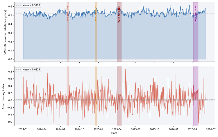
Figure 1 — VPIN-60 (top) and smart money index (bottom) across 602 NQ sessions, January 2024–June 2026. VPIN shows modest elevations during the Fed Dec and Tariff Apr 2025 episodes (+6%). The SMI is negative during the BoJ shock (late-session selling) and reaches its highest value during the April 2026 tariff episode (late-session accumulation).

Table 1 – Summary Statistics (602 NY sessions, NQ M1 futures)

Metric	Mean	Std Dev	Min	25%	Median	75%	Max
VPIN-60 [0,1]	0.523	0.028	0.452	0.503	0.522	0.539	0.617
Flow imbalance [-1,+1]	0.021	0.056	−0.185	−0.016	0.024	0.061	0.158
Trade intensity (winsorized)	1.005	0.234	0.505	0.848	0.969	1.135	1.632
Smart money index	0.023	0.251	−0.643	−0.142	0.015	0.179	0.866
Flow momentum	0.004	0.131	−0.495	−0.079	0.003	0.093	0.404
Flow confidence [0,1]	0.650	0.182	0.000	0.675	0.711	0.727	0.792

The VPIN distribution warrants comment before the regime analysis. The total range across 602 sessions is 0.45 to 0.62 — a spread of 0.17 points around a center of 0.52. This narrow distribution confirms that M1 bar aggregation substantially suppresses the volume imbalance signal, as anticipated in the introduction. Each one-minute NQ bar contains hundreds of individual executions; the buy and sell volumes within each bar are nearly balanced in aggregate, even when the net directional pressure over the session is meaningful. The VPIN_OHLC function is included because it is the best available approximation at bar resolution and produces directionally correct elevations during stress, but users should not treat the absolute values as probabilities.

Flow confidence averages 0.650. Forty sessions (6.6%) receive confidence = 0 due to jump contamination from Part 4. The remaining 68.4% of sessions exceed 0.70, meaning the flow signal is gated as reliable for approximately two-thirds of the sample.

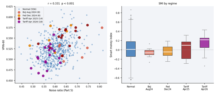
Figure 2 — Left: VPIN-60 against noise ratio (Part 5) across 602 sessions (r = 0.331, p < 0.001). Sessions with elevated noise also tend to have higher VPIN, consistent with the interpretation that noise and informed flow are not independent at M1 resolution. Right: smart money index by regime. The BoJ shock is the only regime with a negative median SMI, indicating late-session selling. The April 2026 tariff episode shows the strongest late-session buying.

Table 2 – Regime Comparison (602 sessions)

Regime	Sessions	VPIN-60	vs Normal	Flow imbalance	SMI	Flow confidence
Normal	556	0.522	—	0.021	0.021	0.653
BoJ shock (Aug 2024)	8	0.523	+0.2%	0.010	−0.062	0.434
Fed Dec (Dec 2024)	6	0.553	+5.9%	0.028	−0.033	0.576
Tariff Apr 2025	14	0.554	+6.0%	0.008	0.013	0.656
Tariff Apr 2026	18	0.506	−3.2%	0.031	0.147	0.690

Three findings from the regime table connect directly to the earlier articles in the series.

First, the BoJ shock raises VPIN by only +0.2% above normal. This is despite it being the highest-volatility episode in Part 5 (noise ratio 0.677) and the second-highest in Part 4 (23.8% annualized). This dissociation suggests that the BoJ carry-trade unwind was a volatility event without a corresponding increase in informed directional flow — consistent with a liquidation cascade where all participants are selling simultaneously rather than an informed-versus-uninformed trade. The SMI of −0.062 supports this interpretation: late-session selling continued through the close, with no evidence of informed accumulation.

Second, the April 2025 tariff shock shows VPIN +6% above normal alongside a flow imbalance near zero (0.008) and an SMI near zero (0.013). Elevated VPIN with near-zero directional imbalance is consistent with high two-sided volume — the market is active but neither buyers nor sellers are dominant. This matches the Part 4 finding of inverse leverage during the tariff shock: when both sides are equally aggressive, there is no net directional pressure.

Third, the April 2026 tariff episode shows VPIN below normal (−3.2%) alongside the highest SMI in the dataset (0.147). Below-normal VPIN with positive SMI is a distinct pattern: the session is quiet overall, but late-session participants are systematically accumulating. This may be consistent with the cross-paper finding in Parts 4 and 5 that markets appear to have adapted to the tariff regime — informed participants are positioned, not reactive.

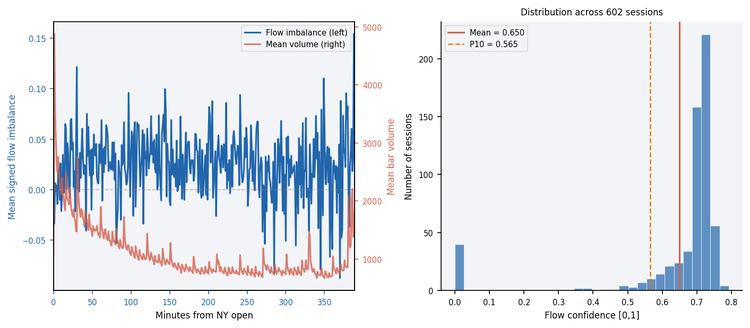
Figure 3 — Left: intraday signed flow imbalance (blue, left axis) and mean volume (red, right axis) by minute from NY open. Flow imbalance is near zero at the open and rises modestly through the session, consistent with noise-dominated early trading and increasing directional clarity later. Right: distribution of flow confidence across 602 sessions. The spike at confidence = 0 represents the 40 jump-contaminated sessions.

Limitations

The OHLCV limitations documented in Part 5 apply with equal force here. The key additional limitation specific to Part 6 is that VPIN_OHLC() is not the Easley-López de Prado-O'Hara VPIN. The canonical VPIN requires volume buckets of fixed size; the bucket construction ensures that each observation represents the same quantity of market participation regardless of clock time. VPIN_OHLC() uses fixed time bars, which means that low-volume bars and high-volume bars contribute equally to the imbalance calculation. On NQ M1, this produces the narrow VPIN distribution (0.45 to 0.62) documented in the empirical section.

The Smart Money Index is sensitive to the choice of n_ends — the number of early and late bars used in the calculation. The default of 15 bars is calibrated to the NQ M1 NY session structure, where the first 15 minutes capture the opening noise and the final 15 minutes capture the closing institutional flow. Users applying the function to other instruments or session structures should recalibrate n_ends accordingly.

Trade intensity requires a pre-computed baseline. The baseline warming-up problem — the first 20 sessions produce inflated values — is inherent to any ratio-based intensity measure and cannot be avoided without discarding early data. The function header documents this limitation and recommends verifying that the baseline exceeds a meaningful value before using the result.

The theoretically correct implementation path uses volume buckets or dollar buckets as described by López de Prado (2018) and implemented for the MQL5 platform by Njoroge (2026). Bucket-based aggregation eliminates the time-bar bias in these metrics and produces VPIN values with the statistical properties the Easley et al. (2012) framework requires. The functions in this article are the best available OHLCV approximations and are appropriate for live indicators without tick access.

Practical Thresholds

All thresholds are derived from the empirical distribution across 602 NQ M1 sessions (January 2024–June 2026). They are heuristic operational cutoffs, not formal hypothesis-test critical values, and are specific to this instrument and sample period.

Metric	Threshold	Basis	Interpretation	Action
VPIN-60	> 0.559	90th pct	Strong volume imbalance	Reduce position; widen stops
VPIN-60	> 0.539	75th pct	Elevated imbalance	Increase caution; monitor closely
Flow imbalance	> 0.092	90th pct	Strong buyer pressure	Consider aligning with flow direction
Flow imbalance	< −0.055	10th pct	Strong seller pressure	Consider aligning with flow direction
Trade intensity	> 1.13	75th pct	Elevated activity; flow signal more reliable	Increase weight on flow metrics
Trade intensity	< 0.85	25th pct	Quiet session; flow signal less reliable	Discount flow metrics; rely on vol
SMI	> 0.330	90th pct	Strong late-session accumulation	Consider long bias for next session
SMI	< −0.293	10th pct	Strong late-session distribution	Consider short bias for next session
Flow confidence	< 0.565	10th pct	Noise or jumps contaminate signal	Do not trade on flow metrics alone
Flow confidence	= 0	—	Jump-contaminated session	Do not use any flow metric

//--- Example: full signal combining Parts 4, 5, and 6
RobustFractalAnalysis  rfa;
MicrostructureAnalysis msa;
VolatilityAnalysis     va;
OrderFlowAnalysis      ofa;

PopulateHurstAnalysis            (Symbol(), PERIOD_M1, 90, rfa);
PopulateVolatilityAnalysis       (Symbol(), PERIOD_M1, 90, va, rfa);
PopulateMicrostructureAnalysis   (Symbol(), PERIOD_M1, 90, msa, rfa);
PopulateOrderFlowAnalysis        (Symbol(), PERIOD_M1, 90, ofa, msa, va,
                                  vol_baseline);  // caller pre-computes baseline

//--- Gate: only trade when flow is reliable
if(ofa.flow_confidence < 0.565) return;  // P10 threshold

//--- Select direction from flow imbalance and SMI
double direction = 0.0;
if(ofa.flow_imbalance > 0.092 && ofa.smart_money > 0.0)
   direction = +1.0;  // buyer pressure + late accumulation
else if(ofa.flow_imbalance < -0.055 && ofa.smart_money < 0.0)
   direction = -1.0;  // seller pressure + late distribution

if(MathAbs(direction) < 0.5) return;  // no aligned signal

//--- Volatility-targeted sizing (Part 4)
double current_vol = (msa.noise_ratio < 0.632)
                      ? va.realized_vol : va.figarch_vol;
double target_vol  = 0.0004;
double base_pos    = (current_vol > DBL_MIN_POSITIVE)
                      ? target_vol / current_vol : 1.0;

//--- Scale by confidence and trade intensity
double intensity_scale = MathMin(1.5,
                                  MathMax(0.5, ofa.trade_intensity));
double position = direction * base_pos
                   * ofa.flow_confidence * intensity_scale;

Folder Structure and Include Path

All Part 6 functions are added to the existing foundation header. No new files are created. The folder structure remains unchanged from Parts 1–5:

MQL5\
└── Indicators\
    └── HurstProfile\
        ├── HurstProfile.mq5
        └── Includes\
            └── MicroStructure_Foundation.mqh

#include "Includes\MicroStructure_Foundation.mqh"

Conclusion

The six functions complete a practical, safe pipeline for extracting order‑flow information from M1 OHLCV when tick data are unavailable. They provide: a directional imbalance proxy (VPINOHLC, directional only), a signed volume flow (OrderFlowImbalance), session activity scaling (TradeIntensity with a 20‑session baseline), intraday informed‑flow detection (SmartMoneyIndex), short‑term acceleration of pressure (OrderFlowMomentum), and a wrapper (PopulateOrderFlowAnalysis) that returns an OrderFlowAnalysis struct.

Crucially, flowconfidence is not cosmetic — it is gated: sessions with jumpintensity above the Part 4 P90 are excluded (confidence = 0), and elevated noise from Part 5 proportionally reduces weight. Practical thresholds (P75/P90) and usage patterns are provided for NQ M1 (VPIN, flowimbalance, SMI, tradeintensity, flowconfidence).

The result is a ready measurement block you can drop into a strategy: compute metrics → apply confidence gate → select direction (flow_imbalance + SMI) → size by volatility and intensity. This offers a disciplined, auditable way to harvest directional information from bar data while avoiding over‑confident trading on microstructure artifacts.

Getting the Source Code via MQL5 Algo Forge

Algo Forge provides Git-based version control in the cloud, so you will always have access to the latest version of the code, including any updates or fixes made after this article was published. The full repository is available at MQL5 Algo Forge.

References

Attached files |

Download ZIP

HurstProfile.mq5 (12.98 KB)

MicroStructure_Foundation.mqh (85.97 KB)

Warning: All rights to these materials are reserved by MetaQuotes Ltd. Copying or reprinting of these materials in whole or in part is prohibited.

This article was written by a user of the site and reflects their personal views. MetaQuotes Ltd is not responsible for the accuracy of the information presented, nor for any consequences resulting from the use of the solutions, strategies or recommendations described.

References

- Easley, D., López de Prado, M.M. & O'Hara, M. (2012). Flow toxicity and liquidity in a high-frequency world. Review of Financial Studies, 25(5), 1457–1493.
- Kyle, A.S. (1985). Continuous auctions and insider trading. Econometrica, 53(6), 1315–1335.
- Lee, C.M.C. & Ready, M.J. (1991). Inferring trade direction from intraday data. Journal of Finance, 46(2), 733–746.
- López de Prado, M.M. (2018). Advances in Financial Machine Learning. Wiley.
- Njoroge, P.M. (2026). Beyond the Clock (Part 1): Building Activity and Imbalance Bars in Python and MQL5. MQL5 Community Articles.