Defining your Edge (Part 1): Using a Discrete Fourier Transform and a Spiking Neural Network in a Trading Robot

Introduction

It can be argued that trading systems today suffer from data bloat or the over-reliance on correlated, lagging indicators. In order for one to develop an edge therefore, this research series introduces a diverse library of special algorithm-neural network pairings. We launch off with an unusual hybrid union: a Discrete Fourier Transform cycle decoder that we marry to a biological Leaky Integrate-and-Fire Spiking Neural Network. We are after isolating hidden market frequencies.

The Fourier-SNN Pairing

This pairing of the Fourier Transform and Spiking Neural Network (SNN) is intended to give us a non-correlated edge via spectral decomposition and a time based confirmation. While traditional indicators often lag from static lookbacks, the Fourier engine acts as a cycle decoder that dynamically scans past price or indicator data in order to separate the dominant frequency wave. This is thus able to transform metrics such as MACD and RSI into predictive wave functions that identify key turning points before they visually unfold.

The SNN rules execution timing by bringing time and pressure metrics to the mix. Rather than generating immediate noisy trade signals with static weights, the inputs are treated as synaptic stimulation that charges a digital membrane's potential energy. This potential energy leaks away when momentum stalls but accumulates when several market variables align over consecutive bars. So, a trade is only triggered when the accumulated "voltage" exceeds a strict threshold, thus generating an execution spike. This ensures that cyclical reversals are verified by sustained momentum before capital is used.

The pairing's ideal Setting

Trading systems are bound to fail when market regimes change for instance, a shift from a trending market to a ranging one. This can highlight the need to have a diverse library of customized strategies. The Fourier Transform and Spiking Neural Network (SNN) hybrid particularly target market-phases that are in transition. This is attempted by the Fourier Transform decoding the dominant cycle length to filter out whipsaws, while the SNN prevents overacting to short-term price spikes by mandating validation over several bars to ensure the entry signals are valid at the final time of execution, when sufficient "voltage" has been accumulated. 

Algorithm and Network Definition

The case for this combination

Regular models that combine Moving Averages and say, classical networks can be a bit brittle and reactive. In contrast, the Discrete Fourier Transform (DFT) and Spiking Neural Network (SNN) seek to balance mathematical precision and time based validation. If we were to visualize the market as a turbulent ocean, the DFT would be playing the role of a submarine sonar, ignoring superficial surface storms in order to accurately map out hidden, rhythm based tide waves deep underwater. The SNN function for its part would be that of a disciplined torpedo commander, waiting patiently on each incoming sonar ping to build up internal pressure. With this build up, a trade is only triggered when a strict preset threshold is cleared.

Math Formulae

In order to do a proper analysis and deconstruction of the operational design of our hybrid trading engine, it may be good to move past metaphors by formalizing the mathematical equations that govern both the algorithm and neural network. This hybrid model is anchored on two primary formulae: the Discrete Fourier Transform (DFT) for spectral decomposition and the Leaky Integrate-and-Fire (LIF) differential approximation for temporal neural compute.

The Spectral Engine:

We treat the market's rolling price history as a finite, discrete time-series vector x[n] of length N, where n stands for the discrete time or bar index (n = 0, 1, ... N-1). The Discrete Fourier Transform changes this spatial price vector into a frequency domain spectrum X[k], where every complex coefficient is linked to a distinct harmonic frequency index k:

Where:

• X[k] is the k-th complex frequency coefficient (the output represents phase and amplitude of the k-th harmonic frequency).
• k is the discrete frequency index (k = 0, 1, ..., N-1), for the cyclic harmonic being studied.
• sum from {n=0} to {n=N-1} stands for the discrete summation over the entire rolling historical data window, by index.
• N is the total window size for the number of historical data points being transformed.
• n is the discrete time index (spanning from n = 0, 1, ..., N-1), that identifies each candlestick in history.
• x[n] is the spatial input value at index n (the raw price data, MACD line value, or RSI line value at that exact bar).
• j is the imaginary unit constant, defined as the square root of [-1]. (often denoted as i).
• e is Euler's number (approx: 2.71828), serving as the base of the natural logarithm in projecting exponential complex growth.
• 2pi/N is the angular frequency step, that normalizes the geometric distribution of the wave cycles.

If we apply Euler's formula we would be able to decompose this complex equation into its real and imaginary cartesian portions, which can be worked out sequentially by using discrete summations.

Where:

• Re(X[k]) is the real portion of the k-th complex frequency coefficient.
• Im(X[k]) is the imaginary part of the $k$-th complex frequency coefficient.
• sum from {n=0} to {n=N-1} represents the discrete total that loops and aggregates calculations for every bar over the sample history.
• N is the total sample length (the fixed number passed into the algorithm).
• n is the discrete space index (n = 0, 1,... , N-1), identifying the particular position in a lookback window.
• x[n] is the spatial input data value at index n (raw price, or  MACD or RSI value).
• k is the discrete frequency index (k = 1, 2, ..., (N/2)-1), for the cyclic wave frequency being calculated.
• (2pi k n)/N is the angular phase argument, that sets the geometric point on a circle evaluated for bar n at frequency k.
• -(Negative Sign) is the math convention used with imaginary summation to keep phase alignment according to Euler's formula.

For every component of frequency k, the magnitude or amplitude A[k], stands for the structural strength of that particular cycle, within a historical price window and this is derived by the Pythagorean theorem as follows:

The phase angle phi[k] that gives us the current positional shift of the wave relative to time's origin, is computed with this two-argument arctangent formula:

Once the engine loops through all the frequencies up to the Nyquist limit (N/2), we are able to isolate the dominant frequency component k_dom, that has the maximum amplitude A[k]. This continuous math projection of the dominant wave over the rolling time array is worked out to forecast the current cycle state y_pred with this expression:

Where:

•  y_pred is the continuous cyclical predicted value that is normalized strictly within a bounded range of [-1.0, 1.0], and represents the theoretical location of the market wave.
• phi[k_dom] is the isolated phase shift angle (got from 'MathArctan2') of our dominant cyclic frequency component. It anchors the wave's true starting position relative to history timelines.
• k_dom is our dominant frequency harmonic index that has the maximum spectral amplitude we got in the Fourier summation sweep.

This is able to normalize the final cycle output to be within a bounded range of [-1.0, 1.0], and this represents an absolute cyclical trough and peak respectively.

The Neural Engine:

The Spiking Neural Network depends on an algorithmic adaptation of the biology-based Leaky Integrate-and-Fire neuron. Whereas regular neurons map inputs straight to outputs via a static activation function, a LIF neuron handles inputs as if they were temporary electrical charges that change their time-dependent inner state variable that we refer to as the membrane-potential (V_m). In continuous time, this membrane's potential dynamics are ruled by a first-order linear differential equation:

Where:

• tau_m is a membrane time constant (tracked in milliseconds with, tau_m = R x C_m), this determines how quickly the internal voltage passive-leaks back toward its baseline resting potential.
• V_m(t) is the time-based membrane potential of the neuron at time t. It represents the piled-up inner electrical voltage.
• dV_m(t)/dt is the first derivative of the membrane potential with respect to time. It tracks instantaneous rate of voltage change.
• -(Negative Sign) is the "mathematical-force" driving the leak; this ensures that without active input currents, the membrane potential naturally decays towards zero.
• R is the total membrane resistance, which sizes-up how heavily incoming pre-synaptic electrical currents physically affect the inner potential.
• I(t) is the time-varying total pre-synaptic input current at time t (or the arrays passed from indicators and Fourier engine).

In our discrete-time algorithmic implementation (we have every discrete step mapping to a new candlestick bar), we estimate this continuous leakage by engaging a discrete decay factor gamma. This gamma is rangebound [0, 1] and is controlled by the input parameter 'InpSnnDecay'. Our updating rule for the membrane potentials of the Buy and Sell neurons (V_buy and V_sell) is formalized as:

Where:

• V_m[t] is the current membrane potential of the neuron at the present time or candlestick bar t.
• V_m[t-1] is the past membrane potential of the neuron from the immediately prior time step (t-1). It acts as the baseline memory state.
• gamma is the discrete leak factor ('InpSnnDecay'). It is bounded [0, 1], and sets the percentage of voltage lost per bar.
• (1 - gamma) is our retention multiplier, setting the fraction of the prior membrane potential that is kept within the current step.
• sum from {i=1} to {i=M} is the discrete summation operator mapping over all M unique incoming signals (M=3 in our full hybrid model).
• M is the total number of independent pre-synaptic input sources feeding into the network.
• w_i is the static synaptic weight given to input channel i (e.g., w_1 = 0.6, w_2 = 0.4, w_3 = 0.5). This scales its physical impact on the potential.
• S_i[t] is the normalized value of the pre-synaptic input signal from channel i at the bar t.

The neuron evaluates this accumulated inner voltage against a strictly set firing threshold (the V_th) that we control with the input parameter 'InpSnnThreshold'. The step-activation function that creates actionable post-synaptic spike H[t] is defined as follows:

Importantly, when a post-synaptic spike happens (H[t] = 1), the neuron would trigger an instantaneous reset. This would purge its inner state back to the baseline value in order to prevent runaway positive feedback loops. This reset thus follows the equation below.

The complete mathematical framework changes simple historical numeric arrays into a highly coordinated system capable of measuring structural market cycles while filtering through time based neural conviction.

MQL5 Implementation

Transitioning from theory/exploration to practical application involves carefully translating our model of spectral and neural engines into a strict MQL5 syntax. What follows is an elaborate, line-by-line dissection of the custom Expert Advisor. We not only paste code; we examine its structure given the hybrid arrangement we have between DFT and SNN, and try to lay out the case of how it processes raw market data into high-conviction trade executions.

Environment Setup

The basis of most robust trading robots could arguably lie in how they manage their state environment. We are putting together a trade robot and not an Expert Advisor, as the latter, if coded in MQL5, could be one that references MQL5's built in base classes in the files 'Expert.mqh' and 'ExpertBase.mqh'. We are doing most of the work "from scratch". We are purposefully avoiding the sometimes bulky, rigid structure that can be used with the 'CExpert' framework. This framework can at times obscure raw execution that we would need for our custom neural processing. Instead we are choosing a hybrid procedural architecture, that uses the built-in 'CTrade' and 'CSymbolInfo' classes solely for execution and stability. We retain absolute control over the 'OnTick()' function loop. At the center of our Trade Robot is the 'EMode' enumeration. This acts as a neurological switchboard. It allows the user to separate components of the algorithm before using the hybrid system.

//--- Enums for EA Operation Modes
enum EMode
  {
   MODE_FOURIER_PRICE = 0,       // 1. Fourier Transform on Raw Price Cycles
   MODE_FOURIER_MACD = 1,        // 2. Fourier Transform on MACD Turning Points
   MODE_FOURIER_RSI = 2,         // 3. Fourier Transform on RSI Turning Points
   MODE_FOURIER_COMBINED = 4,    // 4. Combined Fourier (Price + MACD + RSI)
   MODE_PRICE_ACTION_SNN = 5,    // 5. Pure Price Action & Candlestick via SNN
   MODE_INDICATOR_PATTERN = 6,   // 6. Indicator Pattern Recognition (Divergences) via SNN
   MODE_HYBRID_FULL = 7          // 7. Full Hybrid (Fourier Cycle Filtering + SNN Setup)
  };

By switching modes when testing, a developer can separate when a failure in the equity curve is because of Fourier cycle miscalculating a phase or is caused by the SNN misinterpreting the momentum. In 'OnInit()', we initialize our 'ExtTrade' class, setting out important safety parameters like the slippage and the Magic Number where the later could allow the flexibility in managing not just Trade Robot positions but also manual entries. Crucially, the execution loop in 'OnTick()' starts with a strict time barrier: <code: if(timeCurrentBar == timeLastBar) return;/> . Given that our Transform and discrete LIF network calculate structural shifts, basing on completed data periods, running this heavy computation on every micro-tick would bring in a lot of processing bloat and false neural spikes.

Indicator Choice

Before we look at the details in the two engines, let us touch on the rationale behind the pre-synaptic simulation that is fed into the neural network. Why are we using the MACD and RSI oscillators? The Fourier engine spots 'when' a cycle could turn, but it does not measure the physical market force behind every turn. Ideally we would have to use secondary metrics to validate the wave structure. The Relative Strength Index (RSI) was chosen since it is range-bound to [0, 100] . It tracks extreme spatial exhaustion. At the start of a Fourier engine cycle trough, an RSI reading in the oversold region would give us spatial confirmation. The Moving Average Convergence Divergence (MACD) is also chosen because it is structurally unbound. By measuring the derivative of momentum - the acceleration or deceleration of a trend, we are able to compute divergences. These would be the gap between the MACD line and the zero-line. This gives us a raw directional velocity. 

Thus, when combined - the bounded exhaustion (RSI), and the unbounded velocity (MACD), our fundamental frequency wave (Fourier) creates a non-correlated triad. If all three align, the mathematical probability of a successful reversal becomes significantly higher than depending on one metric.

The Fourier Transform Algorithm

Our function 'CalculateFourierTurningPoint()' is the sonar engine of this system. It breaks down a rolling historical data array to identify the "dominant frequency" responsible for the prevalent price action.

//+------------------------------------------------------------------+
//| Mathematical Engine: Discrete Fourier Transform (DFT)            |
//+------------------------------------------------------------------+
double CalculateFourierTurningPoint(double &data[])
  {
   int N = ArraySize(data);
   if(N == 0)
      return 0.0;

This function requires an input data array of size N, as set by the input parameter 'InpFourierWindow'. Mathematically, N should be a power of 2 (e.g. 32, 256, 512... ) in order to avoid frequency leakage and ensure a stable discrete processing. Zero value is not allowed.

   double max_amplitude = 0.0;
   double dominant_phase = 0.0;
   int dominant_k = 1;

We then proceed to initialize our tracking variables. The engine's main objective is to find the frequency index 'k' that gives the highest amplitude, and thus represents the bulkiest dominant cycle within the array.

   for(int k = 1; k < N / 2; k++)
     {
      double real = 0.0;
      double imag = 0.0;

The outer loop iterates over the frequency gamut. We begin at k = 1 to intentionally skip the DC component k = 0, that stands for the static average of the data and gives no cyclical insight. We conclude at N/2 that is the Nyquist limit; any frequency analyzed beyond half the window size would lead to aliasing and data distortion.

      for(int n = 0; n < N; n++)
        {
         double angle = 2.0 * M_PI * k * n / N;
         real += data[n] * MathCos(angle);
         imag -= data[n] * MathSin(angle);
        }

The inner loop of this Discrete Fourier Transform, listed above, implements Euler's formula. For every specific frequency 'k', we scan all the individual bars 'n' in the historical window. We then multiply the spatial price data 'data[n]' by the Cosine and Sine of the proportional angle to decompose the signal into its constituent Real and Imaginary vectors.

      double amplitude = MathSqrt(real * real + imag * imag);
      if(amplitude > max_amplitude)
        {
         max_amplitude = amplitude;
         dominant_phase = MathArctan2(imag, real);
         dominant_k = k;
        }
     }

By using the Pythagorean theorem on Real and Imaginary vectors, we are able to work out the 'amplitude' or strength of the frequency 'k'. When this amplitude is found to be the highest, we log this. Importantly, we use 'MathArctan(imag, real)' to extract the 'dominant_phase' the precise geometric shift that shows where the cycle currently sits relative to its starting point.

   return MathSin(dominant_phase + (2.0 * M_PI * dominant_k * (N - 1) / N));
  }

Finally, we rebuild the wave by projecting the dominant frequency 'dominant_k' forward to the most recent bar '(N - 1)' and adding the 'dominant_phase' shift. We map the result through a Sine wave. This helps normalize the output strictly to be between [-1.0, 1.0] the absolute cycle bottom and absolute cycle top respectively 

The Spiking Neural Network

If the Fourier Transform is the sonar, thanks to 'CalculateFourierTurningPoint()', then 'EvaluateSpikingNeuralNetwork()' is our torpedo commander. This function manages the biological concept of 'membrane potential', over a given period. 

//+------------------------------------------------------------------+
//| AI Engine: Leaky Integrate-and-Fire Spiking Neuron Model         |
//+------------------------------------------------------------------+
int EvaluateSpikingNeuralNetwork(double inputSignal1, double inputSignal2, double inputSignal3)
  {
   static double w1 = 0.6, w2 = 0.4, w3 = 0.5;
   static double membranePotentialBuy = 0.0;
   static double membranePotentialSell = 0.0;

The most crucial keyword here is 'static'. Since we are defining the membrane potentials as static variables, they get to be preserved through the termination of the 'OnTick() loop'. This is the explicit memory network. The variables 'w1', 'w2', and 'w3' handle the synaptic weights. These weights set how heavily the network favors the Fourier wave (w1) as opposed to the secondary indicators. 

   membranePotentialBuy  *= (1.0 - InpSnnDecay);
   membranePotentialSell *= (1.0 - InpSnnDecay);

What we have listed above is the "Leaky" aspect of the LIF network. Prior to evaluating any new data, the network would forget a proportion of its past conviction by using the input 'InpSnnDecay'. When this decay is 0.2, the potential loses 20% of its power for each price bar. This prevents the network from triggering a trade by basing on obsolete or stale momentum.

   if(inputSignal1 > 0)
      membranePotentialBuy  += inputSignal1 * w1;
   else
      membranePotentialSell += MathAbs(inputSignal1) * w1;

The network works out the inputs next. When 'inputSignal1' (Fourier cycle) is above zero (thus trending towards a peak), it would excite the Buy neuron's membrane potential. If on the other hand it is negative then its absolute value would excite the Sell neuron. We multiply the input by its weight 'w1'. We repeat this in similar fashion for 'inputSignal2' and 'inputSignal3'.

   bool buySpike = (membranePotentialBuy >= InpSnnThreshold);
   bool sellSpike = (membranePotentialSell >= InpSnnThreshold);
   if(buySpike && !sellSpike)
     {
      membranePotentialBuy = 0.0;
      return 1;
     }
   if(sellSpike && !buySpike)
     {
      membranePotentialSell = 0.0;
      return -1;
     }
   return 0;
  }

This network checks its own tension. It determines whether the accumulated potential has crossed the input 'InpSnnThreshold' level. When a 'buySpike' happens, the network immediately returns '1' (a buy signal) this would lead to the membrane potential being aggressively reset to 0.0. This Biology-reset sees to it that the Trade Robot only fires one clean order per structural alignment. This averts the runaway grid executions when we have sustained trends.

Connecting the Engines

Arguably, the real power of this model is realized when we engage 'ExecuteHybridFull()'. This function merges the math isolation of the Fourier Transform with the time-based conviction of the SNN

//+------------------------------------------------------------------+
//| Generates a hybrid trading signal                                |
//| Uses Fourier and RSI rules or an optional SNN with MACD input    |
//| Returns: 1 = buy, -1 = sell, 0 = no signal                       |
//+------------------------------------------------------------------+
int ExecuteHybridFull()
  {
   double closePrices[];
   ArrayResize(closePrices, InpFourierWindow);
   if(CopyClose(_Symbol, _Period, 0, InpFourierWindow, closePrices) < InpFourierWindow)
      return 0;
   double fourierPriceSignal = CalculateFourierTurningPoint(closePrices);

The first thing we do is capture the pure raw price-data and forward it through our Fourier engine. The parameter 'fourierPriceSignal' would now hold a value between -1.0 and 1.0, and this would represent the isolated frequency phase of the market.

   double rsiValues[], macdValues[];
   ArrayResize(rsiValues, 5);
   ArrayResize(macdValues, 5);
   if(CopyBuffer(hRSI, 0, 0, 5, rsiValues) < 5)
      return 0;
   if(CopyBuffer(hMACD, MAIN_LINE, 0, 5, macdValues) < 5)
      return 0;
   double rsiMomentum  = rsiValues[0] - rsiValues[4];
   double macdMomentum = macdValues[0] - macdValues[4];

Following this, we pull a short 5-bar array of our technical indicators. By subtracting the historical reading '[4]' from the present reading '[0]' , we get to work out the real velocity vector - 'rsiMomentum' and 'macdMomentum'.

   if(InpUseSNN)
     {
      return EvaluateSpikingNeuralNetwork(fourierPriceSignal, rsiMomentum, macdMomentum);
     }

To wrap this up, we inject these three distinct calculated realities into our Spiking Neural Network. Thus the pure mathematical phase shift, the bounded spatial momentum, and unbound velocity, all get combined to build a "neural-pressure" over time.

Trade Execution and State Management

Building a good signal would be fruitless if the execution logic it uses is fragile. This being a Trade Robot and not an MQL5 'Expert Advisor' where this logic is defined by the MQL5 library classes, our 'ManagePositions()' function gets to play a pivotal role. It serves as the physical interface between our SNN and the broker's server. By using the Standard Library's 'CTrade' and 'CSymbolInfo' objects, we get to bypass the need for using 'MqlTradeRequest' data structures. 

//+------------------------------------------------------------------+
//| Position management using CTrade class                           |
//+------------------------------------------------------------------+
void ManagePositions(int signalType)
  {
   ExtSymbolInfo.RefreshRates();
   bool hasOpenPosition = false;
   int totalPositions = PositionsTotal();

In this function, we start off by calling the 'ExtSymbolInfo.RefreshRates()' method. This is a critical step that ensures our bid/ask prices are well synchronized with the server and this should avert order-rejection from slippage. 

   for(int i = totalPositions - 1; i >= 0; i--)
     {
      ulong ticket = PositionGetTicket(i);
      if(ticket != 0 && PositionGetString(POSITION_SYMBOL) == _Symbol && PositionGetInteger(POSITION_MAGIC) == InpMagicNumber)
        {
         long type = PositionGetInteger(POSITION_TYPE);
         //--- If signal is opposite to position type, close it
         if((type == POSITION_TYPE_BUY && signalType == -1) ||
            (type == POSITION_TYPE_SELL && signalType == 1))
           {
            ExtTrade.PositionClose(ticket, InpSlippage);
            ExtTrade.PrintResult();
           }
         else
           {
            //--- Position aligns with signal; no action needed
            hasOpenPosition = true;
           }
        }
     }

Our state management listed above, iterates backward through any open positions. This strictly filters for the chart symbol '_Symbol' as well as the used magic number 'InpMagicNumber'. When the SNN brings a -1 (Sell) spike when a long position is in place, the Trade Robot would use 'ExtTrade.PositionClose()' to exit this trade. This would be a dynamic reversal since the system depends mostly on cyclical nature of the Fourier wave as opposed to the static hard-coded stop losses. 

   if(!hasOpenPosition)
     {
      if(signalType == 1)
        {
         double price = NormalizeDouble(ExtSymbolInfo.Ask(), ExtSymbolInfo.Digits());
         if(!ExtTrade.Buy(InpLotSize, _Symbol, price, 0.0, 0.0))
           {
            PrintFormat("Buy failed. Ask=%G error=%d", price, GetLastError());
           }
        }
      else
         if(signalType == -1)
           {
            double price = NormalizeDouble(ExtSymbolInfo.Bid(), ExtSymbolInfo.Digits());
            if(!ExtTrade.Sell(InpLotSize, _Symbol, price, 0.0, 0.0))
              {
               PrintFormat("Sell failed. Bid=%G error=%d", price, GetLastError());
              }
           }
     }
  }

When the environment is clear of conflicting trades, the 'CTrade' class manages the entries by automatically using the preset standard deviation as well as lot sizes.

Initial Testing Sandbox

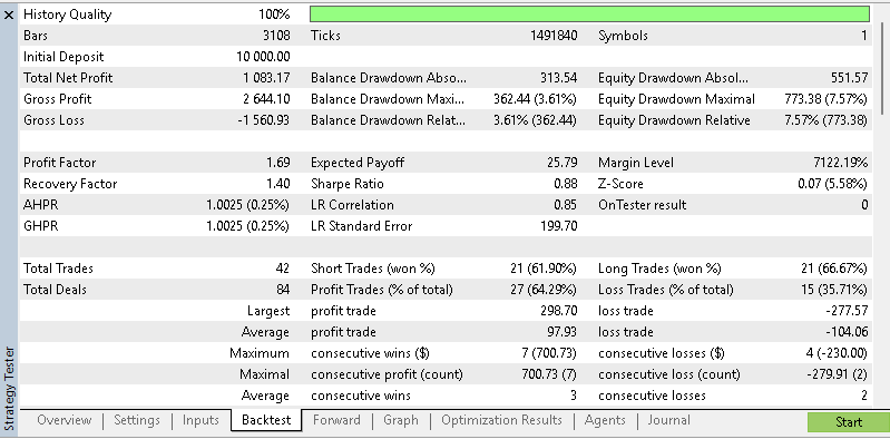
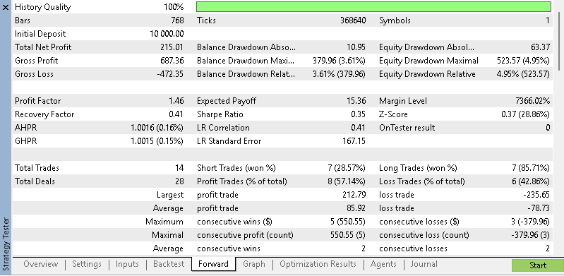
Implementing our hybrid model in MetaTrader 5's Strategy Tester needs some patience because throwing arbitrary parameters at the wall and expecting something to stick i.e., getting an upward linear trend in the equity curve would be foolhardy. Our system needs to be carefully tuned to particular volatility regime of the picked asset. Therefore in setting up the optimization matrix, the primary interplay is between the Fourier frequency resolution ('InpFourierWindow') and the network's biological memory ('InpSnnDecay'). For our optimized testing we are selecting the forex pair GBPJPY on the 2-hour timeframe. We optimize from 2025.01.01 to 2026.01.01. We then do a forward test from 2026.01.01 to 2026.05.01. The key parameters that we are tuning are 'InpFourierWindow', 'InpSnnThreshold', and 'InpSnnDecay'.

This grid setup ensures the trader is able to cover a spectrum from fast, highly reactive networks (those with low threshold and high decay) all the way to highly convicted trend-filtering system (high thresholds, low decay). This ensures the test run inherently makes the network adept to the three main market regimes: bullish trend, bearish phase, and consolidation period. 

Post-Optimization Test Results Analysis

The ideal input settings from our optimization run were able to profitable forward walk. The best inputs called for a 90-bar Fourier window and an aggressive 82% neural membrane decay meaning our system filtered noise immediately, synchronizing momentum to fire.

Below is a combined equity curve from running the test over the optimization and forward walk periods.

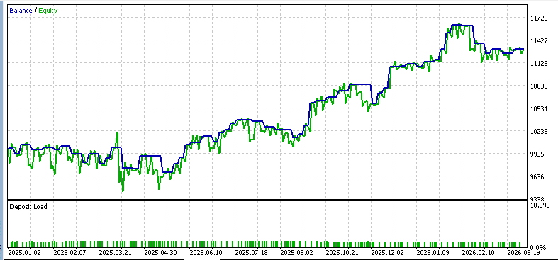
This very strict logic limited us to 56 trades and yielded a 62.5% win rate and 41,305.70 profit on a $10,000 account. This hybrid model where we tuned for whether or not to use the network as a secondary gate, also gave us a profit factor of 1.64 and an equity drawdown that did not exceed 7.57%

Summary

Conclusion

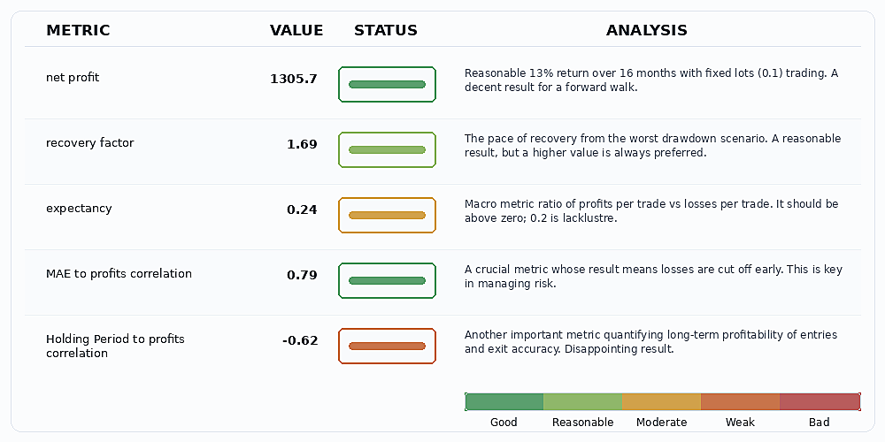
The 16-month test validates our Fourier-SNN edge, to a degree. As always, extra testing with other symbols and over wider periods is recommended. However by routing cyclical wave data through a temporal gateway, the hybrid engine seems to have been able to filter out localized market noise. Future variations of this model can explore dynamic synaptic plasticity (STDP) for adaptive weighting; Radix-2 FFT migration in an effort to reduce the compute lag to O(N log N); as well as volatility-scaled membrane decay.

name	description
01 Fourier SNN RSI MACD.mq5	Trade Robot that implements model
i.set	Test Optimization Inputs